Peter Beerli

Talk: Analysis of genomic sequence data using finite sites models

Tutorial: Population model selection using a combination of VCF and reference data

I will assume that the users of the tutorial, know some basic UNIX commands, such as the bash or zsh shell, that they can run python 3 scripts and either can compile my program Migrate on their computer or have a Mac or Linux machine. Window may work, but I cannot guarantee that I manage to have the latest MIgrate binary available (although the current one will work [I think]).

Overview of the activity:

This tutorial discusses the use of migrate-n for model selection.
We assume that you have a genomic data set in VCF format and a reference sequence; as an example we use a small dataset using a VCF dataset contemporary human populations . We use a VCF of two African population of, the reference is chromosome 23.
We need python3 to extract and combine the VCF with the reference sequence and generate a migrate-n dataset. In the future this will be incoroporated into migrate-n, but currently we need to preprocess. Our handling of the VCF data is also rather rudimentary (if you want to use your VCF data with migrate-n and conversion fail, contact us so that we can fix the translation script).
To successfully run the tutorial in short time, we would need a cluster computer; we will shortcut some of the steps, and also give hints how to troubleshoot problems.
A first run of migrate, we will discuss how to specify models for migrate-n; we will explain the layout of the output.
Migrate-n uses Bayesian model comparison using marginal likelihoods, in the last few minutes of the tutorial we will compare a few simple models that were run with human dataset.

Installation

if you downloaded the bbcamp.zip file and unpacked the file you should see a directory migrate-4.5 and tutorial directory. This file is part of the tutorial

Tutorial

Learning goals: students are able to generate a migrate input file from a VCF data file, and can specify different population genetic models and compare them in a Bayesian model selection approach.

Preparing your dataset

I added a simple VCF dataset to the tutorial directory, I suggest that we use this dataset for our tutorial. The tutorial should work the same way with your own dataset, if the conversion step does not fail.

Currently the VCF dataset option does not exist in migrate. In future version you will be able directly to use VCF data, but for now we have a python script to convert the VCF data into a migrate format.

vcf2mig --help

will deliver

syntax: vcf2mig --vcf vcffile.vcf <--ref ref1.fasta,ref2.fasta,... | --linksnp number >  <--popspec numpop ind1 ind2 .... | --pop populationfile.txt> --out migrateinfile
  --vcf vcffile : a VCF file that is uncompressed or .gz, currently only
                  few VCF options are allowed, simple reference
                  and alternative allele, diploid and haploid data
                  can be used
  --ref ref1.fasta,ref2.fasta,... : reference in fasta format
                  several references can be given, for example for
                  each chromosome, if this option is NOT present then
                  the migrate dataset will contain only the SNPs
  --linksnp number : cannot not be used with --ref; defines linkage groups of snps
                  for example in a VCF file covering 10**9 sites, a value of 100000
                  will lead to 10 linked snp loci, if this option and the --ref are
                  are missing, then the resulting dataset will contain single, unlinked snps
  --popspec numpop ind1,ind2,... : specify the population structure, number of populations
                  with the number of individuals for each population
                  This option exlcudes the option --pop
  --pop popfile:  specify a file that contains a single line with
                  numpop ind1,ind2 in it
                  This option exlcudes the option --popspec
  --out migratedatafile:  specify a name for the converted dataset in migrate format

Example:
vcf2mig.py --vcf vcffile.vcf.gz --ref ref.fasta --popspec 2 10,10 --out migratefile
vcf2mig.py --vcf vcffile.vcf --popspec 3 10,10,10 --out migratefile
vcf2mig.py --vcf vcffile.vcf --linksnp 10000 --popspec 2 5,10 --out migratefile

You specified:['/Users/beerli/bin/vcf2mig.py', '--help']

There are two main modes of the script. (1) generate complete sequence using a reference to fill in the missing sites; (2) just use the VCF data to generate a SNP dataset.

(1) Full reference sequence

This will allow to use phylogenetic style mutation models, such as JC69, F84, HKY, and Tamura-Nei inlcuding Gamma-deviated site rate variation. This will result in rather different analyses than the ones you would do with Site Frequency Spectra, which seems to be the common analysis route when we have large amounts of genomic data. This allows to consider finite sites mutation models that are more appropriate for analyses than the “infinite sites” or the *no mutation" mutation model.

We call the script like this:

vcf2mig.py --vcf 1.vcf.gz --ref 1.fasta --popspec 2 5,5 --out infile.1

But before we run the script we peek into the raw VCF file and the reference sequence to get an idea what we need to do, here the first few lines of the VCF file (1.vcf.gz – if you want to look yourself use for example emacs or zless because the file is compressed and your editor needs to know that:

##fileformat=VCFv4.2
##source="VCF   simulated   by  momi2 using msprime backend"
##contig=<ID=chr1,length=1000000>
##FORMAT=<ID=GT,Number=1,Type=String,Description="Genotype">
##INFO=<ID=AA,Number=1,Type=String,Description="Ancestral   Allele">
#CHROM  POS ID  REF ALT QUAL    FILTER  INFO    FORMAT  YRI_0   YRI_1   YRI_2   YRI_3   YRI_4   CHB_0   CHB_1   CHB_2   CHB_3   CHB_4
chr1    16  .   A   T   .   .   AA=A    GT  1|0 0|0 1|0 1|0 1|0 0|0 0|0 0|0 0|0 0|0
chr1    23  .   A   T   .   .   AA=A    GT  1|1 1|1 1|1 1|1 1|1 0|0 0|0 0|0 0|0 0|0
chr1    38  .   A   T   .   .   AA=A    GT  0|0 0|0 0|0 0|0 0|0 1|1 1|1 1|1 1|1 1|1
chr1    43  .   A   T   .   .   AA=A    GT  1|1 1|1 1|1 1|1 1|1 0|0 0|0 0|0 0|0 0|0

The VCF file is rather simple with reference and alternative allele, my script ignores the Ancestral Allele specification, it recognizes the diploid (or haploid) data case and uses the header file to get the names of the individual in the data, here we have 5 individual with YRI and 5 with CHB stem, we recognize these as two populations, each has 5 diploid individuals each.

The reference file needs to be standard FASTA file, it can contain multiple entries, for example for each chromomose, our example has only a single chromosome, and give that the VCF we use comes from a simulator (momi2) the file looks weird and contains only ‘A’ as the reference sequence, your real data will look different. Note: I believe that this matters and actually can deliver different results because the mutation models would pick up base frequency differences. Here the first few bytes of the FASTA reference file:

> chr1
AAAAAAAAAAAAAAAAAAAAAAAAAAAAAAAAAAAAAAAAAAA.....

We then call your script [the current version is very picky about spelling and the two dashes (–)]:

vcf2mig.py --vcf 1.vcf.gz --ref 1.fasta --popspec 2 5,5 --out infile.1

where the option –popspec gives the number of populations and the number of individuals.

This will generate a file that contains the data; but is not yet ready to analyze, the first few lines look like this:

 2 1 Translated from VCF 2020-07-28
# VCF file used:      1.vcf.gz                   
# Reference file:     1.fasta                    
# Migrate input file: infile.1                   
(s1000000)                           
 10 Pop1                             
0YRI_0:1   AAAAAAAAAAAAAAAATAAAAAATAAAAAAAAAAAAAAAAAAATAATAAA...
1YRI_0:2   AAAAAAAAAAAAAAAAAAAAAAATAAAAAAAAAAAAAAAAAAATAATAAA...
2YRI_1:1   AAAAAAAAAAAAAAAAAAAAAAATAAAAAAAAAAAAAAAAAAATAATAAA...
3YRI_1:2   AAAAAAAAAAAAAAAAAAAAAAATAAAAAAAAAAAAAAAAAAATAATAAA...
...
9YRI_4:2   AAAAAAAAAAAAAAAAAAAAAAATAAAAAAAAAAAAAAAAAAATAATAAA...
 10 Pop2                             
0CHB_0:1   AAAAAAAAAAAAAAAAAAAAAAAAAAAAAAAAAAAAAATAAAAAAAAAAA...
1CHB_0:2   AAAAAAAAAAAAAAAAAAAAAAAAAAAAAAAAAAAAAATAAAAAAAAAAA...
2CHB_1:1   AAAAAAAAAAAAAAAAAAAAAAAAAAAAAAAAAAAAAATAAAAAAAAAAA...
...

The infile.1 would force migrate run analyze for each individual 1 million sites, although this is actually possible, it may not be desirable because it would be treated as a single locus (on my Macbook Pro late 2016 with 16 GB RAM the datasets runs with defaults in about 7 minutes using 660MB memory because most of the sites are aliased). The data was simulated with a recombination rate larger than zero. migrate has a shortcut the handle large genomic data by specifying a set of equidistant loci along the genome, so we can specify 10, 100, or any arbitrary number of loci out of the complete dataset. The shortcut takes the instruction of the number of sites 2 1 Translated from VCF 2020-07-28

(s1000000)

and replaces it with (for example)

[25o21000](s1000000)

and you also need to change the number of loci on the first line: the first number is the number of populations and the second number is the number of loci:

  2 1 Translated from VCF 2020-07-28

becomes

  2 25 Translated from VCF 2020-07-28

This specifies 25 loci that are each 21000 base pairs long. and once migrate runs this converts to

(0s21000) (40000s21000) (80000s21000) (120000s21000) (160000s21000) (200000s21000) (240000s21000) (280000s21000) (320000s21000) (360000s21000) (400000s21000) (440000s21000) (480000s21000) (520000s21000) (560000s21000) (600000s21000) (640000s21000) (680000s21000) (720000s21000) (760000s21000) (800000s21000) (840000s21000) (880000s21000) (920000s21000) (960000s21000)

These individual loci can be specified by hand if needed. Our dataset is now ready! migrate is a Bayesian inference program that uses Markov chain Monte Carlo to deliver a posterior probability density of the parameters of interest. With many loci this can be a very frustrting process because the runtime depends on the number of individuals, the number of populations, and the number of loci. If we need for a single locus 7 minutes, this translates to quite some time for, say, 1000 loci. migrate can be run in parallel using standard MPI interfaces, such as OPENMPI or MVAPICH2. Using a large number of parallel running CPUs cuts down the time considerably. I often run large datasets on our cluster using 501 CPUs to analyze 500 loci in parallel; this cuts down runtime even on laptops with multiple cores.

(1) SNP data set without a reference sequence

If we are not interested to reconstitute the complete sequence, we can simply translate the VCF variant calls to a SNPS (currently there is no quality control possible) We can call the script like this:

vcf2mig.py --vcf 1.vcf.gz --linksnps 100000 --popspec 2 5,5 --out infile.2

or like this:

vcf2mig.py --vcf 1.vcf.gz --popspec 2 5,5 --out infile.2

The first variant creates linke snps, the example combines all snps that are in position 0-100000, 100001-200000, … into groups, the example data has a million sites, thus the command generates 10 loci with completely linked snps. The second variant generates unlinked snps. I am not sure how usefule this is because the example generates >100,000 single snp loci, which will take a ver long time to run, and since the migrate uses random coalescences among individuals this seems not to be the best use of computing power because a single snp has a rather boring simple tree. with two groups (here: all individual with A and all individuals with T), thus, migrate spends a large amount of time to change trees that are inconsequential with the data. [I will not have time to discuss snps in depth and will stick to the reference sequence approach.]

Setting up a population model

migrate uses an adjacancy matrix to define the interactions among populations.

Defaults

The defaults in migrate are to estimate all population sizes \(\Theta\) and all immigration rates \(M\) independently.

For example a 3-population model where all populations A, B, and C exchange migrants at individual rates can be specified like this:

	A	B	C
A	x	x	x
B	x	x	x
C	x	x	x

Of course, this is not all that informative, but it is the default.

Specifying models without divergence

There are many ways to specify different structured models, migrate has a set of options to help with that:

x or ‘*’ means that this parameter is estimated
0 means that this parameter is not estimated (works only on off-diagonal elements)
s means the migration parameter is symmetric, this implies that \(M_{1\rightarrow 2} = M_{2\rightarrow 1}\)
c means that the value is constant and not estimated, the values needs to be specified in the the start-parameter option
m means take the average of all parameters labeled m, \(\Theta\) and \(M\) will be treated separately. A matrix full of m will be a two- parameter model (all populations share the same values for 1 \(\Theta\) and 1 \(M\)).
there are upper case variants for s and m (S, M) that use instead of the migraiton parameter \(M\) the number of immigrants \(Nm\). I n most cases this is not a good choice because \(\Theta\) and \(Nm\) are more strongly correlated than \(\Theta\) and \(M\).
all other lower alphabet letters except c, d, t, m, s, t, and x can be used to form groups of parameters (similar to m but more flexible), see example.

More examples:

	A	B	C
A	x	0	x
B	x	x	0
C	0	x	x

	A	B	C
A	e	b	a
B	a	e	b
C	0	a	x

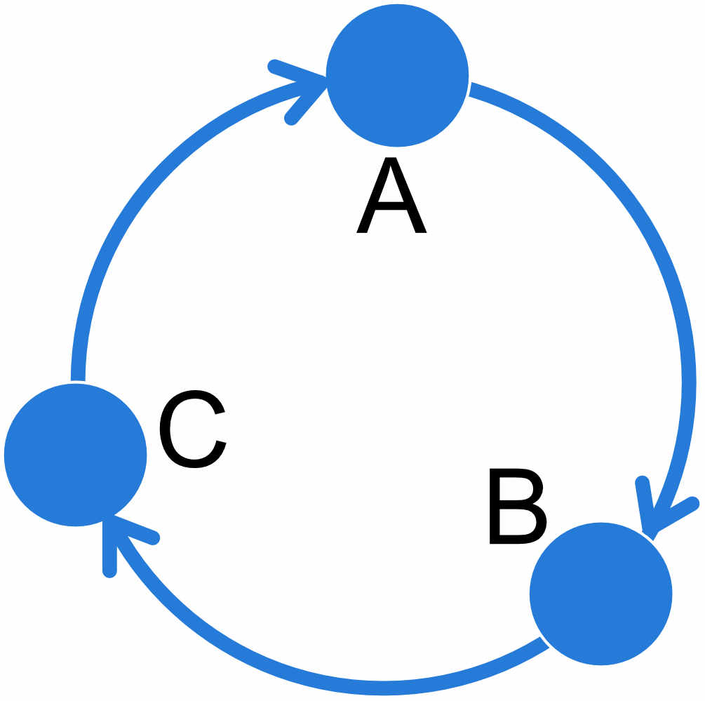
REMINDER: the populations specified on the row of the adjanceny matrix are the receiving populations, populations on the columns are the sending populations, thus in the circular unidrectional stepping stone example above, population A receives migrants from population C and we estimate the parameter \(M_{C\rightarrow A}\), population B receives migrants from population A and we estimate \(M_{A\rightarrow B}\) etc.

Answer these questions

Click on the question to reveal the answer, but write down the answer before you peek :-).

1. specify the matrix for a 2-population system with unidrectional migration from 2 \(\rightarrow\) 1

custom-migration={** 0*}

2. specify a migration matrix for a 5-population system where population 1 and 5 are on a mainland, population 2 is and island close to 1, population 4 is close to 5, and population 3 is far out in the sea but closest to 2. ‘Close’ means reachable by rafting, and once on an island it will be difficult to get off again.

custom-migration={*000* **000 0**00 000** *000*}

Specifying models with divergence

For the divergence specification we also use the adjancency matrix. For example if we have a model where the populations do not exchange migrants we could specify the matrix like this

	A	B	C
A	x	0	0
B	d	x	0
C	0	d	x

d means divergence from the ancestral column population
D means divergence from the ancestral column population with onpoing immigration
t means divergence time is the same for all the matrix elements with the t.

	A	B	C
A	x	0	0
B	D	x	0
C	0	D	x

Migration is problematic and models with immigration and divergence may need additional ancestral populations to allow the estimation to be identifiable. Here an example that needs ancestral population to get better estimates of divergence and migration.

	A	B	C	D
A	x	0	0	0
B	0	x	x	t
C	0	x	x	t
D	d	0	0	x

migrate has a menu to enter this adjancency matrix, but given the many options it may seem easier for complex scenarios to edit the parameter file (it is a text file) directly. the option is named custom-migration and contains the adjancency matrix, for example the example from above looks like this

custom-migration={ x000 0xxt 0xxt d00x}

If a diagonal element is set to zero the program will crash! There are also models that will not work well or fail. All models essentially need to be able to end in one common ancestor, for example we may be tempted to code an admixture example like this

	A	B	C
A	x	0	0
B	d	x	d
C	0	0	x

but this will not work well because we force to have two roots, and this can lead to failures during the run, one can code this better as this (a) or this (b)

(a)	A	B	C
A	x	0	0
B	d	x	d
C	d	0	x

More complicated than (a) is this (b) model that forces a sequence of divergences. Both models should deliver similar values so, although (b) will estimate a population size for population D.

(b)	A	B	C	D
A	x	0	0	0
B	d	x	d	0
C	0	0	x	d
D	d	0	0	x

Answer these questions

1. specify the matrix for two current populations A, B that share a common ancestor C

custom-migration={*0d 0*d 00*} or custom-migration={*0t 0*t 00*}

2. If the first questions is answered using ’d' what does that mean for the divergence times?

Specifying ’d' instead of ’t' allows the two current populations to have splits from the ancestor at different times.

Run a model selection exercise

We will have little time so we try to run two examples:

using the parmfile specified in the tutorial it uses a model that is coded as
```
1 Pop1           * 0 t 
2 Pop2           0 * t 
3 ancestor       0 0 * 
```
run it using: migrate-n parmfile #do not change the menu
Once it is done rename the outfile and the outfile.pdf, for example outfile-x0t0xt00x and outfile-x0t0xt00x.pdf
run another parmfile, for example: migrate-n parmfile-x0dx

we can compare the marginal likelihoods of these two runs, there is a small python script that helps with calculating the numbers, but that can be done “by-hand”, too: [I forgot to add the python script bf.py in the tarball; you can then get with this command: wget https://peterbeerli.com/downloads/scripts/migbf.zip; you will need to unzip it and then can use it like this:

grep “All ” outfile* | sort -n -k 4,4 | python bf.py

and it will produce something like this:

Model	Log(mL)	LBF	Model-probability
1:exampleruns/outfile-x0t0xt00	-167828.22	0.00	1.0000
2:exampleruns/outfile-xd0x:	-167966.92	-138.70	0.0000
3:exampleruns/outfile-x0dx:	-168043.88	-215.66	0.0000
4:exampleruns/outfile-xxtxxt00	-180387.23	-12559.01	0.0000
5:exampleruns/outfile-xxxx:	-236426.20	-68597.98	0.0000