00 Basics: input files, a first run, and the output
Draft: work in progress. This recipe is not finished yet; sections may be incomplete and results may change.
Status: draft (2026-11-10). Tested with migrate-n 7.0.106 and 6.1.82.
This recipe runs Migrate with its default settings on four small simulated data sets: one and two populations, DNA sequences and microsatellites. It explains the input files, the menu, the parmfile, and every file a run writes. Because the data are simulated, we know the true values and can check the estimates.
Contents
- What you need
- The data sets and their true values
- The infile: sequences
- The infile: microsatellites
- The menu and the parmfile
- Running Migrate
- The output files
- Reading the results
- Did the run work? Convergence
- One population vs. two, DNA vs. microsatellites
- Running in parallel (MPI)
- What next
1. What you need
- migrate-n (Migrate 7 or 6.1); see the README of the source tree for
installation. Check the version with
migrate-n -version. - This folder. Everything below is run from
cookbooks/00-basics. - Optional: Python 3 with msprime, numpy, to re-create the data
(
scripts/simulate_basics.py).
2. The data sets and their true values
| File | Marker | Populations | Loci | Samples |
|---|---|---|---|---|
data/dna-1pop.txt | DNA, 500 bp per locus | North | 5 | 10 sequences |
data/dna-2pop.txt | DNA, 500 bp per locus | North, South | 5 | 10 sequences each |
data/msat-1pop.txt | microsatellites | North | 5 | 10 diploid individuals |
data/msat-2pop.txt | microsatellites | North, South | 5 | 10 diploid individuals each |
All four come from one population history, simulated with msprime: North has an effective size of 25,000 and South of 12,500. Forward in time, each generation a fraction 1e-5 of North’s individuals arrive from South, and a fraction 4e-5 of South’s individuals arrive from North. The one-population data sets contain only North, without migration.
Migrate does not estimate population sizes and migration fractions directly,
but scaled by the mutation rate mu: Theta = 4 Ne mu and M = m / mu. The
mutation rate differs between the markers (1e-7 per site and generation for
the DNA, 5e-5 per locus and generation for the microsatellites), so the true
values differ too (data/truth.txt):
| Parameter | DNA | Microsatellites |
|---|---|---|
| Theta_1 (North) | 0.01 | 5 |
| Theta_2 (South) | 0.005 | 2.5 |
| M_2->1 (into North from South) | 100 | 0.2 |
| M_1->2 (into South from North) | 400 | 0.8 |
| 4 Ne m into North = Theta_1 M_2->1 | 1 | 1 |
| 4 Ne m into South = Theta_2 M_1->2 | 2 | 2 |
The number of immigrants per generation (4 Ne m) does not depend on the mutation rate, so it is the same for both markers.
Migrate’s migration rates are always immigration rates: M_2->1 is the rate at which individuals of population 1 arrive from population 2, forward in time.
3. The infile: sequences
The first lines of data/dna-2pop.txt:
2 5 basics DNA 2pop simulated
(s500) (s500) (s500) (s500) (s500)
10 North
Nor00     GATAATTAGTTTAATTATTACCCGCAAATTGCCTCCAATGATTCCCATAGTCG...
Nor01     GATAATTAGTTTAATTATTACCCGCAAATTGCCTCCAATGATTCCCATAGTCG...
...
10 South
Sou00     GATAATTAGTTTAATTATTACCCGCAAATTGCCTCCAATGATTCCCATAGTCG...
- Line 1: number of populations, number of loci, and a title.
- Line 2: the length of each locus,
(s500)= 500 sites. Every individual’s line holds all loci one after the other (here 5 x 500 = 2500 bases). - Then for each population: the number of samples and the population name,
followed by one line per sample: a name of exactly 10 characters (padded
with blanks;
nmlengthin the parmfile changes the width) and the sequence. Missing data:?orN; gaps:-. - Give every sample a unique name across the whole file: assignment and haplotyping find individuals by name.
4. The infile: microsatellites
The first lines of data/msat-2pop.txt:
2 5 . basics msat 2pop simulated
10 North
Nor00     18.19 20.20 23.24 22.23 18.18
Nor01     17.19 20.20 22.28 23.23 18.23
...
10 South
Sou00     19.18 20.21 22.28 21.23 16.16
Line 1: number of populations, number of loci, the character that separates the two alleles of a diploid individual (
.), and a title.For each population: the number of individuals and the population name, then one line per individual with a 10-character name and one genotype per locus.
18.19means alleles with 18 and 19 repeats. Missing alleles:?.Alleles are repeat numbers. If you have fragment lengths instead, add a line with the repeat length of each locus directly after the first line, where sequence data have the line with the locus lengths (a missing entry repeats the previous one); Migrate then converts fragment lengths to repeat numbers:
2 5 . basics msat 2pop with fragment lengths
#@M 2,2,4,4,2
10 North
...
5. The menu and the parmfile
Migrate reads its settings from a file called parmfile in the current
directory. Without a parmfile it uses the built-in defaults. Start it with
the data file named infile (or a parmfile that names your data file) and
you see the main menu (full screens: menu/*.txt):
  =============================================================
  MAIN MENU
  =============================================================

  D       Data type currently set to: DNA sequence model
  I       Input/Output formats and Event reporting
  P       Parameters  [start, migration model]
  S       Search strategy
  W       Write a parmfile
  Q       Quit the program

  To change the settings type the letter for the menu to change
  Start the program with typing Yes or Y
===>
D(menu/data.txt): data type and mutation model. Sequences default to F84 with base frequencies from the data; our DNA was simulated under the simpler Jukes-Cantor model, so our parmfiles setdatamodel=JC69.I(menu/input-output.txt): data file name, random seed, output file names, logfile.P(menu/parameters.txt): start values and the migration model. The default is the full model: every population has its own Theta, and every pair of populations exchanges migrants in both directions.S(menu/search.txt): the MCMC run (chain length, burn-in, heating, replicates) and the priors.Wwrites all current settings intoparmfile;Ystarts the run.
The menu is good for exploring the options. For real work write the parmfile
once with W, edit it with a text editor, and run with -nomenu; then the
parmfile documents exactly what was run. Every option in the parmfile is
explained in the comment lines above it.
Our parmfiles (parmfiles/parmfile.*) are the default parmfile with only
these lines changed (scripts/make_parmfiles.sh makes them):
datatype=SequenceData          # BrownianData for the microsatellites
datamodel=JC69                 # DNA only: the model used for the simulation
infile=dna-2pop.txt
random-seed=OWN:20261107       # a fixed seed: the run can be repeated exactly
logfile=YES:logfile
bayes-file=YES:bayesfile
bayes-allfile=YES:1:bayesallfile
title=00-basics dna-2pop
heating=YES:1:POWER:5          # 5 chains instead of the default 4, see below
menu=NO
The settings you will look at most often, with their defaults:
| Parmfile line | Default | Meaning |
|---|---|---|
long-inc=100 | 100 | steps between two recorded samples |
long-sample=10000 | 10000 | recorded samples per locus |
burn-in=10000 | 10000 | discarded at the start, in units of the increment: 10000 x 100 = 1,000,000 steps |
heating=YES:1:{1,1.5,3,1000000} | 4 chains | heated chains help the cold chain (temperature 1) move between peaks |
replicate=NO | NO | independent replicates, needed for the Gelman-Rubin check (section 9) |
theta=PRIOR:50, migration=PRIOR:10 | start values: 50% and 10% quantiles of the prior | |
custom-migration={**} | full model | which parameters are estimated, see 01-migration |
Our parmfiles, like all recipes, use heating=YES:1:POWER:5: five chains
with temperatures 1, 2.61, 10.08, 101.59 and 1,000,000 instead of the
default four (1, 1.5, 3, 1,000,000). Section 9 shows how to check whether
the heated chains help.
So a default run records 10,000 samples from 1,000,000 steps per locus,
after a burn-in of another 1,000,000 steps. The menu shows the burn-in as
10000; the outfile shows the steps: Burn-in per replicate (samples*inc): 1000000.
The default priors are uniform and depend on the data type:
| Prior | Sequences | Microsatellites |
|---|---|---|
| Theta | 0 - 0.1 | 0 - 100 |
| M | 0 - 1000 | 0 - 10 |
Our DNA true values lie inside these ranges, but M_1->2 = 400 is not far from the upper bound of 1000; section 8 shows what that does.
6. Running Migrate
migrate-n parmfile -nomenu
or, with this folder’s helper, which copies the data and parmfile into a run directory and times the run:
scripts/run.sh dna-2pop migrate-n runs/dna-2pop
Migrate prints its progress to the screen: the options, a data summary, and for each locus the burn-in and sampling with acceptance ratios and a running effective sample size. With 5 loci the loci run one after the other; with MPI they run in parallel (section 11).
Run times on a Mac (Apple M-series, 16 cores), ten runs at the same time while other programs were also busy, so a single run on an idle machine is faster:
| Data set | 6.1.82 | 7.0.106 |
|---|---|---|
| dna-1pop | 76 s | 71 s |
| dna-2pop | 602 s | 577 s |
| msat-1pop | 113 s | 106 s |
| msat-2pop | 10931 s (182 min) | 10676 s (178 min) |
| msat-2pop, Theta prior 0 - 20 (section 10) | 2710 s (45 min) | 2605 s (43 min) |
With the same seed and parmfile, 6.1.82 and 7.0.106 give the same estimates for these data sets; apart from dates and the version line, the outfiles differ in the wording of one line of the options section, and 7.0.106 prints one extra line.
7. The output files
A run with our parmfiles writes these files:
| File | What it holds | Look at it? |
|---|---|---|
outfile | the results as text: options, data summary, estimates, marginal likelihoods, run diagnostics, warnings | always |
outfile.pdf | the same results with plots of the posterior distributions (12 pages for dna-2pop) | always |
outfile.md | (Migrate 7 only) the results as Markdown with SVG plots, readable on GitHub or in an editor | if you prefer it to the PDF |
logfile | a copy of what was printed on the screen | when something went wrong |
bayesfile | the posterior histograms (1500 bins) for every parameter and locus; locus 6 is the combination over loci | for your own plots |
bayesallfile | every recorded sample of the parameters and the log likelihoods, tab-separated, one line per sample | for trace plots, Tracer, your own analyses |
bayesallfile.ckpt.N | per-locus checkpoint of the marginal-likelihood sums, used by recover=YES | no |
outfile.joint.L.R | summaries of the stored genealogies of locus L, replicate R, used for the joint multi-locus combination | no |
The outfile has these parts, in this order:
- Options in use: what was run, including the priors (table “Prior
distribution”) and the MCMC settings. Check this first. (The line
Theta [Exponential Distribution]refers to the coalescent waiting times, not to the prior: the alternative is the Mittag-Leffler distribution of recipe 08-mittag-leffler.) - Summary of data: loci, sample sizes, and for sequences the number of variable sites per locus. dna-2pop has 13 to 36 variable sites per locus (134 in total).
- Bayesian estimates: one block per locus, then
AllandJoint(section 8). - Monte Carlo error of the joint estimates.
- Marginal likelihoods: needed for model comparison (recipe 05).
- MCMC run characteristics: acceptance ratios, autocorrelation, effective sample sizes (section 9).
- Potential problems: warnings, for example about prior bounds.
The bayesallfile starts with a header (lines starting with #); the data
part is a table:
Steps  Locus  Replicate  lnPost  lnDataL  lnPrbGParam  lnPrior  treeintervals  treelength  Theta_1  Theta_2  M_2_1  M_1_2  ...
100    1      1          132.0   -807.27  939.27       -9.21    46             0.0303      0.00793  0.00300  207.46 236.17 ...
bayes-allfile=YES:1:bayesallfile writes every recorded sample (1); a larger
number writes only every n-th sample and gives a smaller file. For dna-2pop
the file is 9.4 MB.
8. Reading the results
The Bayesian estimates of dna-2pop (Migrate 7.0.106; 6.1.82 gives the same numbers):
Locus Parameter       HPD95lo  HPD50lo     mode  HPD50hi  HPD95hi   median     mean
-----------------------------------------------------------------------------------
    1  Theta_1         0.00240  0.00453  0.00950  0.01693  0.07120  0.01597  0.02323
...
  All  Theta_1         0.00427  0.00573  0.00803  0.00880  0.01340  0.00823  0.00853
  All  Theta_2         0.00127  0.00240  0.00337  0.00440  0.00820  0.00410  0.00445
  All  M_2->1         158.0000 474.6667 494.3333 813.3333 999.3333 607.0000 597.3486
  All  M_1->2          74.6667 136.0000 335.6667 450.6667 950.6667 409.0000 444.2692
Joint  Theta_1         0.00467  0.00753  0.01010  0.01173  0.01740  0.01043  0.01084
Joint  Theta_2         0.00120  0.00193  0.00317  0.00433  0.00807  0.00403  0.00432
Joint  M_2->1          42.0000 196.6667 268.3333 457.3333 876.6667 389.6667 429.2749
Joint  M_1->2         192.6667 630.0000 985.6667 1000.0000 1000.0000 630.3333 615.0504
- Each locus gets its own posterior. A single locus of 500 bp says little: the 95% HPD interval of Theta_1 for locus 1 spans a factor of 30.
Allmultiplies the per-locus posteriors of each parameter on its own.Jointcombines the loci using all parameters together, which is the correct multi-locus posterior. Use the Joint rows. (AJoint*row means the joint estimate is unreliable for that parameter; then use All.)- HPD95lo/HPD95hi: the 95% highest posterior density interval; HPD50 the 50% interval. Report an interval together with the mode or the median.
Compared with the truth:
| Parameter | Truth | Joint median | 95% HPD |
|---|---|---|---|
| Theta_1 | 0.01 | 0.0104 | 0.0047 - 0.0174 |
| Theta_2 | 0.005 | 0.0040 | 0.0012 - 0.0081 |
| M_2->1 | 100 | 390 | 42 - 877 |
| M_1->2 | 400 | 630 | 193 - 1000 |
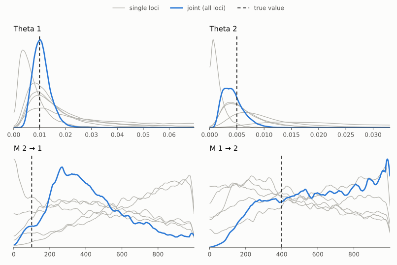
The figure (made with scripts/plot_posteriors.py from the bayesfile)
shows why the loci must be combined: each single locus (gray) gives a broad
posterior, the joint posterior (blue) is much narrower.
The Thetas are estimated well. Five short loci carry much less information about migration: both intervals contain the truth, but they are wide, and the posterior of M_1->2 piles up at the upper prior bound of 1000: its mode is 986 and its 50% HPD interval is 630 - 1000. The outfile warns about it:
Param 4 (Locus 1): Upper prior boundary seems too low!
Param 3 (Locus 2): Upper prior boundary seems too low!
Param 4 (Locus 2): Upper prior boundary seems too low!
Param 3 (Locus 4): Upper prior boundary seems too low!
Param 4 (all loci): Upper prior boundary seems too low!
Most warnings name single loci, but they matter for the joint estimate too (the last line is about the combined posterior): a posterior cut off by the prior bound has a wrong upper limit and a wrong median. More loci would make the M posteriors narrower; with these data, a second run with a wider M prior (for example 0 - 2000) is the right check. Recipe 01-migration deals with this.
One population: dna-1pop gives Theta = 0.0080 (0.0047 - 0.0116), truth 0.01; msat-1pop gives Theta = 4.7 (2.6 - 7.7), truth 5 (Joint medians and 95% HPD intervals).
9. Did the run work? Convergence
A Bayesian MCMC run is only useful if the chain has explored the posterior. Check, in this order:
Effective sample size (ESS) in the outfile, per parameter. Rule of thumb: a few hundred per locus or more. dna-2pop:
Parameter           Autocorrelation   Effective sample size (ESS)
                                                  Sum (*)  Per locus (**)
Theta_1                   0.579                  3423.828         684.766
Theta_2                   0.717                  1958.788         391.758
M_2->1                    0.655                  2747.010         549.402
M_1->2                    0.663                  3028.999         605.800
Genealogies               0.711                  4051.259         810.252
Acceptance ratios: parameter proposals are tuned to about 0.44 (
auto-tune=YES:0.44); genealogy acceptance is usually lower (0.2 here). Very small values (below 0.02) mean the chain hardly moves.The Monte Carlo error table of the joint estimates: a ratio MC error / posterior sd above 0.25 is marked with
*and asks for longer runs. For dna-2pop the ratios are 0.17 - 0.29; Theta_2 (0.29) and M_1->2 (0.26) are marked, so a longer run would sharpen these two estimates.The PDF posterior plots: a smooth, single-peaked posterior is a good sign; a ragged one needs a longer run; a posterior piled up at a prior bound needs a wider prior (section 8).
Replicates:
replicate=YES:3runs three independent chains per locus and withgelman-convergence=YESreports the Gelman-Rubin statistic (sqrt(R) near 1 is good). This costs three times the run time.
The temperatures table at the end of the run shows the heated chains. At
the end of each locus Migrate prints the accepted swaps between neighbouring
chains: for locus 1 of dna-2pop Swap(14418,381,238,...), that is 14418
swaps between the cold chain and the chain at temperature 2.61, 381 between
2.61 and 10.08, and 238 between 10.08 and 101.59. The first number should
not be zero: heated chains that never swap with the cold chain do not help
it. Section 10 shows a run where they did not.
10. One population vs. two, DNA vs. microsatellites
The four runs used the same default settings. They did not work equally well:
| Data set | Run time | ESS per locus | Result |
|---|---|---|---|
| dna-1pop | 71 s | 4221 | Theta 0.0080 (0.0047 - 0.0116), truth 0.01 |
| msat-1pop | 106 s | 658 | Theta 4.7 (2.6 - 7.7), truth 5 |
| dna-2pop | 577 s | 392 - 606 | good Thetas, wide M (section 8) |
| msat-2pop | 178 min | 34 - 49 | not converged, see below |
(ESS per locus: the smallest and largest over the parameters; Migrate 7.0.106.)
Two populations cost more than one: four parameters instead of one, and the genealogies carry migration events, which the MCMC must also sample. Microsatellites with two populations are the hard case here, although Migrate’s Brownian-motion model for microsatellites is fast (about 100 times faster than the stepwise model) and the true values are small: Theta near 5 and M below 1, so Theta x M is 1 and 2. A run is fast as long as Theta x M stays small; the number of migration events in the genealogies, and with it the time per step, grows with Theta x M. A single locus with 20 gene copies says little, and the default prior lets Theta go up to 100 and M up to 10. The chains of msat-2pop spent most of their time far from the truth:
| Locus | samples with Theta_1 M_2->1 + Theta_2 M_1->2 > 100 | samples with a Theta > 20 |
|---|---|---|
| 1 | 76% | 66% |
| 2 | 19% | 26% |
| 3 | 88% | 84% |
| 4 | 59% | 64% |
| 5 | 37% | 59% |
(counted in the bayesallfile). The msat-2pop outfile shows all the warning signs of
section 9:
Parameter           Autocorrelation   Effective sample size (ESS)
                                                  Sum (*)  Per locus (**)
Theta_1                   0.821                   244.936          48.987
Theta_2                   0.923                   171.257          34.251
M_2->1                    0.939                   197.593          39.519
M_1->2                    0.959                   182.531          36.506
Parameter                    Median     MC error   Blocks: lowest  highest  Post. sd   Ratio   Boot err
------------------------------------------------------------------------------------------------------
Theta_1                        5.3659     1.4524     2.2829     9.0654     8.6524   0.168       2.453  * noisy
Theta_2                        1.1626    0.50608     2.2333     4.6678     4.5033   0.112      1.1952  * noisy
M_2->1                          1.818     1.7121     1.6104     9.5246     2.4316   0.704*     1.3907  * noisy
M_1->2                         5.1509    0.88138    0.43577      4.337     2.7299   0.323*     1.9921  * noisy
and all four Joint rows are marked Joint*:
Joint* Theta_1         0.66667  0.93333  4.43333  5.46667 16.13333  5.36667  7.54071
Joint* Theta_2         0.46667  0.53333  0.96667  1.20000  6.40000  1.16667  2.54170
Joint* M_2->1          0.41333  0.35333  0.60333  1.90000 10.00000  1.81667  2.85737
Joint* M_1->2          0.45333  3.68000  0.59667  8.22000 10.00000  5.15000  4.91594
The columns do not even agree with each other: the mode of M_1->2 (0.60) lies outside its 50% HPD interval (3.68 - 8.22), and the 95% interval of M_2->1 starts above its 50% interval. Such a posterior is ragged, with several peaks. The true values are Theta_2 = 2.5, M_2->1 = 0.2 and M_1->2 = 0.8: these estimates are wrong, and the outfile says so.
The heated chains did not help either. The swaps between the cold chain and
the chain at temperature 2.61 were 0, 4, 0, 266 and 3 for the five loci
(Swap(0,21335,45212,...) for locus 1): the cold chain was on its own. With
the default four chains (1, 1.5, 3, 1,000,000) the same run swapped 5,000 -
10,000 times per locus, but did not converge either. Do not report such a
run; run longer, or with replicates, and compare.
A better prior for microsatellites
The data themselves tell how large Theta can be. Under the stepwise mutation
model the variance of the allele sizes in a population is about Theta / 2.
In msat-2pop the variances per locus and population are 1 - 8, so Theta
should be below about 16; a uniform prior from 0 to 20 is generous enough.
parmfiles/parmfile.msat-2pop-theta20 adds one line to the msat-2pop
parmfile:
bayes-priors= THETA * * UNIFORMPRIOR: 0.0 20.0 2.0
(minimum, maximum, and the width of the proposal window).
With this prior the run took 43 minutes instead of 178 (2605 s with 7.0.106, 2710 s with 6.1.82; again both give the same numbers), and the estimates moved toward the truth:
| Parameter | Truth | Theta prior 0 - 100: Joint median (95% HPD) | Theta prior 0 - 20: Joint median (95% HPD) |
|---|---|---|---|
| Theta_1 | 5 | 5.37 (0.67 - 16.1) * | 4.13 (1.39 - 10.1) |
| Theta_2 | 2.5 | 1.17 (0.47 - 6.40) * | 3.17 (0.63 - 5.99) * |
| M_2->1 | 0.2 | 1.82 (0.41 - 10.0) * | 0.91 (0.09 - 4.75) * |
| M_1->2 | 0.8 | 5.15 (0.45 - 10.0) * | 0.88 (0.00 - 8.44) * |
(* = Joint* row: the joint estimate has a large Monte Carlo error.)
With the narrower prior the chains no longer drift to large values: the
share of samples with Theta_1 M_2->1 + Theta_2 M_1->2 > 100 fell to 1 - 39%
per locus. ESS per locus rose from 34 - 49 to 53 - 136, and all four
intervals now contain the truth. The run is better, but not done: three of
the four Joint rows are still marked Joint*, the Monte Carlo error ratios
of Theta_1 and M_2->1 are 0.30 and 0.58, the cold chain swapped only 21 -
347 times per locus, and the outfile still warns about the M prior bound for
loci 1 and 3. Five microsatellite loci from 10 individuals
per population carry little information about migration. The next steps
would be a longer run (long-inc), replicates (replicate=YES:3), or,
best, more loci.
The lesson: look at your data before you accept the default prior. For microsatellites the default Theta prior (0 - 100) is wide on purpose, so that it fits many data sets; for a given data set a narrower prior based on the allele-size variance is both faster and better.
DNA vs. microsatellites: the parameters are on different scales because the mutation rates differ (section 2), but the number of immigrants, 4 Ne m = Theta x M, is comparable. For dna-2pop the joint medians give 0.0104 x 390 = 4.1 into North (truth 1) and 0.0040 x 630 = 2.5 into South (truth 2); with 5 short loci, 4Nm is the least certain quantity. Recipe 01-migration shows how to estimate it directly.
11. Running in parallel (MPI)
The MPI version, migrate-n-mpi, runs the loci in parallel. One process is
the master that collects the results; the others each run a locus:
mpirun -np 6 migrate-n-mpi parmfile -nomenu # 5 loci + 1 master
dna-2pop with 6 processes took 118 s (7.0.106) and 126 s (6.1.82), each run alone on the Mac. The serial runs of section 6 took 577 s and 602 s, but they shared the machine with nine other runs, so the real speed-up is smaller than this ratio. The output files are the same as for a serial run.
The estimates are not identical to the serial run, even with the same seed: each locus draws its random numbers on another process. Both versions agree with each other under MPI (up to the last digit of two marginal-likelihood terms), and the differences to the serial run show how much a 5-locus run varies by chance:
| Parameter | Truth | serial: median (95% HPD) | MPI: median (95% HPD) |
|---|---|---|---|
| Theta_1 | 0.01 | 0.0104 (0.0047 - 0.0174) | 0.0100 (0.0045 - 0.0167) |
| Theta_2 | 0.005 | 0.0040 (0.0012 - 0.0081) | 0.0042 (0.0017 - 0.0080) |
| M_2->1 | 100 | 390 (42 - 877) | 410 (111 - 862) |
| M_1->2 | 400 | 630 (193 - 1000) | 501 (162 - 1000) |
The Thetas hardly change; the poorly determined M estimates move by more.
More processes than loci + 1 do not make a run faster, except with
replicates: replicate=YES:3 gives 15 locus-replicate jobs and can use
16 processes.
12. What next
- 01-migration: migration models, prior choice for M, 4Nm.