01 Migration: migration models
Status: done (2026-11-10). Runs made with migrate-n
7.0.104 (the joint-samples runs with a 7.0.104 build that has the option,
released in 7.0.105), sections 9-10 with 7.0.106; 7.0.105 and 7.0.106
changed only the divergence models.
This recipe uses one simulated data set from three island populations and analyses it with different migration models: every rate free, some rates zero, symmetric rates, and the n-island model. It shows how to write the migration matrix, how to compare the models, and how to choose between M and the number of immigrants 4Nm. Read 00-basics first.
Contents
- The data and the true values
- The migration matrix
- Running the four models
- The full model
- The true model: zero rates
- Symmetric migration and the n-island model
- Which model fits best?
- Better estimates with replicates
- M or 4Nm?
- Priors for M and the window move
1. The data and the true values
Three island populations in a row: Arran, Bute and Coll. Migrants move only
between neighbours (a stepping-stone model); Arran and Coll do not exchange
migrants directly. data/islands.txt has 20 DNA loci of 500 bp and 10
sequences per population, simulated with msprime under the Jukes-Cantor
model (scripts/simulate_migration.py; truth in data/truth.txt):
| Parameter | True value | 4Nm = Theta x M |
|---|---|---|
| Theta_1 (Arran) | 0.01 | |
| Theta_2 (Bute) | 0.01 | |
| Theta_3 (Coll) | 0.005 | |
| M_2->1 (into Arran from Bute) | 100 | 1 |
| M_3->1 (into Arran from Coll) | 0 | 0 |
| M_1->2 (into Bute from Arran) | 200 | 2 |
| M_3->2 (into Bute from Coll) | 100 | 1 |
| M_1->3 (into Coll from Arran) | 0 | 0 |
| M_2->3 (into Coll from Bute) | 200 | 1 |
The loci have 26 to 88 variable sites each. Arran and Coll are the most different populations (average pairwise difference 0.047 per site, against 0.033 for Arran-Bute and 0.037 for Bute-Coll).
2. The migration matrix
The migration model is a matrix in the parmfile, custom-migration, with one
row per population and one column per population. Row i is the receiving
population: the entry in row i, column j is M_j->i, migration into i from j.
The diagonal holds Theta_i. Rows are separated by blanks:
custom-migration={**0 *** 0**}
reads
             from Arran  from Bute  from Coll
into Arran   Theta_1     M_2->1     0
into Bute    M_1->2      Theta_2    M_3->2
into Coll    0           M_2->3     Theta_3
The letters (all listed in the parmfile comments above custom-migration):
| Letter | Meaning |
|---|---|
* | estimated, free |
0 | zero, not estimated |
c | constant: fixed at its start value |
s | symmetric: M_j->i = M_i->j |
S | symmetric number of immigrants: one 4Nm for both directions |
m | mean: all entries marked m share one value (on the diagonal: Thetas) |
M | mean number of immigrants: one 4Nm for all entries marked M |
d, D | population split (recipe 02-divergence) |
The four models of this recipe (scripts/make_parmfiles.sh writes them):
| Model | custom-migration | Parameters |
|---|---|---|
| full | {*** *** ***} | 3 Theta + 6 M = 9 |
| stepstone (true) | {**0 *** 0**} | 3 Theta + 4 M = 7 |
| symmetric | {*s0 s*s 0s*} | 3 Theta + 2 M = 5 |
| island | {mmm mmm mmm} | 1 Theta + 1 M = 2 |
The menu sets the same matrix under P (Parameters), entry 5 Model is set to. The menu does not know the
number of populations yet (it reads the data only after the menu), so type N
and the number first (full screen: menu/model.txt):
  NUMBER OF POPULATIONS = 2

  If the population number is different, type a "N" at the prompt!


  You must give 4 more values out of 4
===> N
  Give the number of populations
===> 3
  NEW NUMBER OF POPULATIONS = 3

  You must now give 9 more values out of 9
===> **0 *** 0**
3. Running the four models
All four parmfiles use the settings of 00-basics: 10000 samples, long-inc 100,
burn-in 10000 samples, and the default uniform priors (Theta 0-0.1, M
0-1000). Heating is heating=YES:1:POWER:5: five chains with the
temperatures 1, 2.61, 10.08, 101.59 and 1000000, spaced as powers so that the
marginal likelihood (section 7) is accurate. With 20 loci this is a moderate
run; the next sections show where it is too short. Each model runs in its
own directory, here with MPI on 15 processes (one master, 14 workers):
for m in full stepstone symmetric island; do
  scripts/run.sh $m migrate-n-mpi runs/$m 15
done
| Model | Parameters | Run time |
|---|---|---|
| full | 9 | 159 min |
| stepstone | 7 | 295 min |
| symmetric | 5 | 11 min |
| island | 2 | 13 min |
(migrate-n 7.0.104 on an Apple M-series Mac. The full and stepping-stone runs shared the Mac with other jobs overnight; the times vary with the load, not only with the model. With replicates, section 8, the stepping-stone model took 43 min.)
scripts/summarize_runs.py prints the numbers used in the next sections for
any run directory: the Joint estimates (median and 95% HPD interval), the starred
rows, the reweighting ESS, the genealogies used per locus, and the marginal
likelihoods:
python3 scripts/summarize_runs.py runs/full runs/stepstone runs/symmetric runs/island
The estimate table of the outfile has the columns HPD95lo, HPD50lo, mode, HPD50hi, HPD95hi, median and mean: the bounds of the 95% and 50% highest posterior density (HPD) intervals, the shortest intervals that hold 95% and 50% of the posterior. The tables below use the median and the 95% HPD interval.
4. The full model
The full model estimates every rate, including the two that are zero in truth. The Joint estimates (median, 95% HPD interval):
| Parameter | True | Joint median | 95% HPD |
|---|---|---|---|
| Theta_1 | 0.01 | 0.0098* | 0.0071-0.0129 |
| Theta_2 | 0.01 | 0.0138* | 0.0104-0.0173 |
| Theta_3 | 0.005 | 0.0044* | 0.0029-0.0059 |
| M_2->1 | 100 | 151* | 61-279 |
| M_3->1 | 0 | 20* | 3-46 |
| M_1->2 | 200 | 180* | 84-311 |
| M_3->2 | 100 | 20* | 0-331 |
| M_1->3 | 0 | 104* | 34-184 |
| M_2->3 | 200 | 242* | 72-481 |
Every row is marked Joint*. The outfile explains the star below the
table: the Joint estimate has a large genealogy-sampling error. The Joint
combination reweights the genealogies sampled for each locus to a common
parameter value; the outfile reports how many genealogies effectively take
part (the “reweighting ESS”). For the full model this is 10, far below the
50 that migrate asks for. The Monte Carlo error table shows the same: the
estimate changes a lot between the four blocks of each chain (M_1->2
between 165 and 410, M_2->3 between 50 and 501).
The chains themselves are fine (ESS 180-360 per locus, acceptance ratios 0.41-0.50). The problem is the number of parameters: with 9 parameters, a few thousand genealogies per locus do not cover the joint parameter space well enough. Do not read these numbers as estimates (the intervals for the two zero rates, M_3->1 and M_1->3, exclude zero); section 8 repeats the run with replicates.
5. The true model: zero rates
The stepping-stone model sets the two Arran-Coll rates to zero and estimates 7 parameters:
| Parameter | True | Joint median | 95% HPD |
|---|---|---|---|
| Theta_1 | 0.01 | 0.0110* | 0.0074-0.0153 |
| Theta_2 | 0.01 | 0.0114* | 0.0069-0.0169 |
| Theta_3 | 0.005 | 0.0060* | 0.0035-0.0081 |
| M_2->1 | 100 | 104* | 23-323 |
| M_1->2 | 200 | 202* | 59-359 |
| M_3->2 | 100 | 104* | 9-315 |
| M_2->3 | 200 | 190* | 69-368 |
The medians are close to the truth and every interval covers it, but all seven rows carry the star (reweighting ESS 45, below 50). Starred rows are not used for the plots and the other tables: they fall back to the All row, the product of the single-locus posteriors. That fallback is visible in the figure: the blue curves are ragged and have several peaks, and some sit far from the truth.
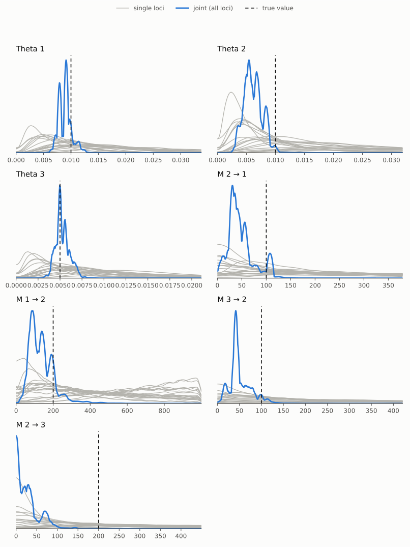
The All rows can be far off. For M_2->3 the All median is 23 (true 200): many single loci have most of their posterior near zero for this rate, and the product of 20 such curves piles up at zero. With a Joint* star, report the Joint value with care and run longer; do not switch to the All value.
6. Symmetric migration and the n-island model
Fewer parameters make the Joint combination easier (reweighting ESS 121 for the symmetric model, 199 for the n-island model), and the stars disappear for the Thetas:
| Model | Parameter | True | Joint median | 95% HPD |
|---|---|---|---|---|
| symmetric | Theta_1 | 0.01 | 0.0092 | 0.0070-0.0114 |
| Theta_2 | 0.01 | 0.0108 | 0.0081-0.0137 | |
| Theta_3 | 0.005 | 0.0066 | 0.0049-0.0082 | |
| M Arran-Bute | 100 and 200 | 146* | 99-203 | |
| M Bute-Coll | 100 and 200 | 127* | 76-193 | |
| island | Theta | 0.005-0.01 | 0.0086 | 0.0075-0.0096 |
| M | 0-200 | 77 | 59-98 |
The symmetric model forces M_1->2 = M_2->1 and M_2->3 = M_3->2. The truth is not symmetric (100 one way, 200 the other), and the estimate falls between the two. The outfile lists a symmetric pair once, under the first name (M_2->1 for Arran-Bute, M_3->2 for Bute-Coll).
The n-island model has one Theta and one M for all populations. Its Theta (0.0086) is close to the average of the three true Thetas (0.0083), and its M (77) is below the average of the six true rates (100), because the two zero rates pull it down. The n-island model answers a different question: how much gene flow is there on average, not between which populations.
7. Which model fits best?
The marginal likelihood, log P(data | model), is in the outfile below the estimates. Use the BTI column (Bezier-corrected thermodynamic integration); it needs the heated chains. The table has one row per locus and two rows for all loci together:
All ... (independent parameters)combines the loci as if every parameter were independent of the others (the method of earlier migrate versions);All ... (joint)uses the Joint combination of section 4, which keeps the parameters together. It is the better value; the outfile gives its Monte Carlo error below the table (joint = ... (MC error ...)).
The short runs:
| Model | Parameters | log ML (BTI, joint) | MC error | Difference to best | Model probability |
|---|---|---|---|---|---|
| symmetric | 5 | -23909.4 | 1.5 | 0 | 0.94 |
| stepstone (true) | 7 | -23912.2 | 1.3 | -2.7 | 0.06 |
| island | 2 | -23932.4 | 0.3 | -22.9 | < 1e-9 |
| full | 9 | -23966.8 | 5.8 | -57.3 | < 1e-24 |
The model probability of model i is exp(lnML_i - lnML_best) divided by the sum of these terms over all models. A log Bayes factor of 2 or more is usually taken as positive support.
- The data reject the n-island model clearly: the populations are not all alike.
- The full model loses 55 log units against the stepping stone. Its extra Arran-Coll rates do not help to explain the data, and the marginal likelihood pays for the extra parameters. The data say the populations form a chain.
- The symmetric model is ahead of the true model by 2.7 log units, about twice the Monte Carlo error. With 20 loci the data cannot tell M = 100 from M = 200 in one direction, and the symmetric model reaches the same fit with two parameters fewer.
The independent-parameters row gives the same order for island and full, but puts the stepping-stone model ahead of the symmetric model by 3.1. When the two rows disagree, use the joint row.
The marginal likelihoods do not need the reweighting ESS of the Joint estimates to be large, and the short runs order the models already. But a single short run is not precise: with replicates (section 8) the values move by up to 9 log units.
The prior range changes the answer
The marginal likelihood is an average of the likelihood over the prior. A
wide prior spreads that average over values the data rule out, and the model
with more parameters pays for each of them: the Occam penalty. The default M
prior, uniform 0-1000, is wide for these data: the Joint intervals of the
stepping-stone and symmetric models stay below 430. The runs of these two
models with four replicates and all genealogies (section 8)
were repeated with M uniform 0-400 (parmfiles parmfile.MODEL-rep4-all-m400,
the same files plus one line):
bayes-priors= MIG * * UNIFORMPRIOR: 0.0 400.0 40.0
| Model | M prior | log ML (BTI, joint) | MC error | Reweighting ESS | Joint* rows |
|---|---|---|---|---|---|
| stepstone (true) | 0-1000 | -23907.8 | 1.3 | 89 | 7 of 7 |
| 0-400 | -23885.5 | 0.5 | 163 | 0 of 7 | |
| symmetric | 0-1000 | -23900.2 | 0.7 | 180 | 0 of 5 |
| 0-400 | -23888.2 | 0.3 | 195 | 0 of 5 |
With the narrower prior the order turns: the true stepping-stone model is ahead by 2.6 log units, against 7.5 behind with the default prior. Both models gain, the stepping-stone model with its four M more (22 log units) than the symmetric model with two (12). These gains are larger than the simple Occam term, log(1000/400) = 0.9 per M parameter: the narrower prior also helps the runs, as the larger reweighting ESS shows.
The stepping-stone estimates with the narrower prior are clean (no star) and close to the truth: Theta 0.0114, 0.0110, 0.0050; M_2->1 83 (32-146), M_1->2 156 (92-241), M_3->2 47 (1-164), M_2->3 255 (130-400); true values 0.01, 0.01, 0.005, 100, 200, 100, 200.
The lesson: Bayes factors depend on the prior. Choose the prior range from what is plausible for the organism, not as wide as possible, and check that the model choice holds for a second reasonable range. Section 10 discusses the M prior.
8. Better estimates with replicates
replicate=YES:4 runs four independent chains per locus, each from its own
random start, and combines them. The parmfiles parmfile.MODEL-rep4 differ
from the short runs only in this line. With MPI, the replicates run on
separate processes, so more processes help: 20 loci x 4 replicates can use up
to 80 workers.
Replicates alone hardly change the Joint estimates. The reason is a limit in
the Joint combination: it uses at most a fixed number of genealogies per
locus, more for models with more parameters (here 16000 for the full model,
10833 for the stepping-stone model, 6111 for the symmetric model and 4000
for the n-island model), however many the run records. With four replicates
each locus records 40000, and most of them are left out. The option
joint-samples sets this number (new in 7.0.105 / 6.1.81):
joint-samples=1        # use every recorded genealogy (a fraction up to 1)
joint-samples=30000    # or a number per locus
joint-samples=AUTO     # the default limit
The parmfiles parmfile.MODEL-rep4-all add joint-samples=1 to the
replicated runs. More genealogies cost time and memory in the Joint
combination: here about 30 MB per locus, harmless for 20 loci, but worth a
thought for hundreds.
The three runs of each model, side by side (Joint* = rows with a large genealogy-sampling error, section 4):
| Model | Run | Genealogies used per locus | Reweighting ESS | Joint* rows | log ML (BTI, joint) |
|---|---|---|---|---|---|
| full (9) | short | 9999 | 10 | 9 of 9 | -23966.8 |
| 4 replicates | 16000 | 18 | 9 of 9 | -23967.2 | |
| 4 replicates, all | 39996 | 16 | 9 of 9 | -23968.6 | |
| stepstone (7) | short | 9999 | 45 | 7 of 7 | -23912.2 |
| 4 replicates | 10833 | 67 | 6 of 7 | -23911.5 | |
| 4 replicates, all | 39996 | 89 | 7 of 7 | -23907.8 | |
| symmetric (5) | short | 6111 | 121 | 2 of 5 | -23909.4 |
| 4 replicates | 6111 | 136 | 2 of 5 | -23903.3 | |
| 4 replicates, all | 39996 | 180 | 0 of 5 | -23900.2 | |
| island (2) | short | 4000 | 199 | 0 of 2 | -23932.4 |
| 4 replicates | 4000 | 199 | 0 of 2 | -23930.4 | |
| 4 replicates, all | 39996 | 200 | 0 of 2 | -23927.8 |
What the table shows:
- With all genealogies the symmetric model is clean: Theta 0.0090, 0.0106, 0.0064 and M 152 (Arran-Bute, 101-206) and 119 (Bute-Coll, 82-161), both between the true rates of 100 and 200.
- The stepping-stone model gains reweighting ESS (45 to 89), but its rows stay starred; its medians (Theta 0.0112, 0.0115, 0.0047; M_2->1 82, M_1->2 153, M_3->2 75, M_2->3 282) are near the truth. The narrower M prior of section 7 removes the stars.
- The full model does not improve: with 9 parameters the reweighting ESS stays below 20, and its Joint values (for example M_1->3 = 12 and M_3->1 = 31, true 0) are not estimates. More loci or much longer chains would be needed; the simpler models are the better answer.
- The marginal likelihoods of the two replicated runs agree within 4 log units; the short runs were off by up to 9. The order holds in all three runs: symmetric ahead of the true stepping-stone model (by 7.5 with all genealogies), then island and full. The data support a chain of populations; with the default prior they cannot show that the rates differ between the two directions (section 7: with M 0-400 they slightly prefer the true model).
Run times (MPI): the replicated runs took 43-50 min on 15 processes with the default limit (250 min for the full model) and 76-132 min on 10 processes with all genealogies (a second Mac), against 11-295 min for the short runs on 15 processes (section 3).
9. M or 4Nm?
Migrate measures migration in two ways:
- M = m / mu, the immigration rate m (the fraction of a population that
arrives from elsewhere each generation) scaled by the mutation rate. This
is the default (
use-M=YES). - 4Nm = Theta x M, the number of immigrants per generation (4 N_i m for
diploid nuclear loci, with N_i the size of the receiving population). In
the outfile it is written as a product, for example
Theta_1*M_2->1for the immigrants into Arran from Bute.
When every rate is free, the two describe the same model and the estimates
can be converted; they differ in what is sampled and therefore in the
prior. use-M=NO samples 4Nm directly, and the MIG prior is then a prior on
4Nm. The letters S (one 4Nm for both directions) and M (one 4Nm for all
entries marked M) always sample 4Nm, also with use-M=YES, because “the
same number of immigrants” is a statement about 4Nm, not about M.
A prior on 4Nm needs a different range. The largest 4Nm the default priors allow is 0.1 x 1000 = 100 (Theta at most 0.1, M at most 1000); that is wide for most organisms. The runs below use uniform 0-20:
use-M=NO
bayes-priors= MIG * * UNIFORMPRIOR: 0.0 20.0 2.0
The true numbers of immigrants of the simulation are 1 (into Arran from Bute), 2 (into Bute from Arran), 1 (into Bute from Coll) and 1 (into Coll from Bute). In M both pairs are asymmetric (100 and 200); in 4Nm the Bute-Coll pair is symmetric (1 and 1), the Arran-Bute pair is not (1 and 2).
The stepping-stone model with use-M=NO (parmfile.stepstone-4nm, 15 min):
| Parameter | True | Joint median | 95% HPD |
|---|---|---|---|
| Theta_1 | 0.01 | 0.0112* | 0.0088-0.0139 |
| Theta_2 | 0.01 | 0.0125* | 0.0093-0.0155 |
| Theta_3 | 0.005 | 0.0052* | 0.0037-0.0068 |
| 4Nm into Arran from Bute | 1 | 0.87* | 0.19-2.09 |
| 4Nm into Bute from Arran | 2 | 1.81* | 1.01-2.88 |
| 4Nm into Bute from Coll | 1 | 0.55* | 0-2.91 |
| 4Nm into Coll from Bute | 1 | 1.30* | 0.69-2.00 |
Every interval covers the truth, but the rows are starred as in the short M run (reweighting ESS 34): the Joint combination needs more genealogies here too (section 8).
The model with symmetric numbers of immigrants, {*S0 S*S 0S*}
(parmfile.symmetric-4nm, 9 min), has no Joint rows. The outfile says
“the joint multi-locus combination does not handle this model yet”: Bute
receives two different shared 4Nm, one from Arran and one from Coll, and
the Joint combination handles at most one shared 4Nm per receiving
population. Only the All row, the product of the single-locus posteriors,
is available:
| Parameter | True | All median | 95% HPD |
|---|---|---|---|
| Theta_1 | 0.01 | 0.0096 | 0.0065-0.0122 |
| Theta_2 | 0.01 | 0.0098 | 0.0069-0.0132 |
| Theta_3 | 0.005 | 0.0056 | 0.0038-0.0075 |
| 4Nm Arran-Bute | 1 and 2 | 1.47 | 1.08-2.16 |
| 4Nm Bute-Coll | 1 and 1 | 0.91 | 0.49-1.16 |
The estimates are close to the truth, but section 5 showed how far the All row can be off; treat it with care.
Marginal likelihoods compare models only under the same prior. A prior of 0-20 on 4Nm is not the same as a prior of 0-1000 on M, so the 4Nm runs cannot be compared with the M runs of section 7. Between the two 4Nm models only the independent-parameters row is available (the symmetric model has no joint row): symmetric 4Nm -23906.1, stepping stone -23911.3. That points to the symmetric model again, but with the cruder row (section 7).
Which one to use: estimate M when the question is about rates (does more gene flow go from A to B than back?), and 4Nm when the question is about the number of migrants or when the prior knowledge is about migrants (for example “at most a few immigrants per generation”).
10. Priors for M and the window move
The M prior
The default M prior is uniform 0-1000. Section 7 showed that the range matters: with M uniform 0-400 the true stepping-stone model is preferred, its Joint estimates lose the stars, and the marginal likelihoods of both models improve. A narrower range costs nothing as long as the posterior stays well inside it, so:
- Run once with a wide prior and look at the posteriors (the gray single-locus curves of the figures and the Joint intervals).
- Set the upper bound a little above the largest value the data support, or from biology: M = m / mu, so an immigration rate of at most 0.001 per generation and a mutation rate of 1e-6 per site and generation give M at most 1000.
- Check that no Joint interval ends at the bound. In the 0-400 runs the interval of M_2->3 ends at 400 (130-400; true 200): 400 is the lowest bound worth trying for these data.
- Compare models only under priors that are reasonable for every model, and check that the choice holds for a second range.
The window move
Besides the moves that change the genealogy or one parameter at a time, migrate has a window move: in one step it changes one migration rate, the population of a few coalescent nodes (the window), and the migration events on the branches attached to them. The topology and the coalescence times stay, so the data likelihood does not change, and a new M does not have to wait for the migration events of the genealogy to follow (details: docs/mcmc_moves_in_migrate.tex, section “The window move”). It is on by default (10% of all moves), and off when it cannot help (one population, no estimated migration rate) or with assignment and haplotyping. The parmfile controls it:
updatefreq= window:0     # turn the window move off
window-delta=0.3         # start width on log M, tuned during the burn-in
window-size=4            # size of the window
The stepping-stone short run without the window move
(parmfile.stepstone-nowindow), against the run of section 5:
| Parameter | ESS per locus, window on | ESS per locus, window off |
|---|---|---|
| Theta_1 | 286 | 166 |
| Theta_2 | 359 | 164 |
| Theta_3 | 311 | 162 |
| M_2->1 | 165 | 47 |
| M_1->2 | 231 | 74 |
| M_3->2 | 226 | 62 |
| M_2->3 | 222 | 48 |
| Genealogies | 456 | 476 |
The window move makes the M chains three to four times more efficient (and the Theta chains about twice) for the same number of steps; the acceptance ratios of the single-parameter moves hardly change (0.41-0.49 against 0.41-0.47), and the window move itself accepts 38% of its proposals. Without it, an ESS of 50 per locus for M is close to the limit where the posterior summaries become unreliable. Keep the default.
One run of each is not enough to compare the Joint combination itself: the run without the window move happened to reach a higher reweighting ESS (77 against 45), but that number depends on how the genealogies of the loci spread, not on how well each chain mixes.
(Sections 9 and 10 were run with migrate-n 7.0.106 on the same Mac, 15 MPI processes: 9, 15 and 8 min.)