02 Divergence: population splits
Draft: work in progress. This recipe is not finished yet; sections may be incomplete and results may change.
Status: draft (2026-11-10), sections 1-9. Sections 3-5 were run with
migrate-n 7.0.104 plus fixes released in 7.0.105 (window move with d
splits, Joint marginal likelihood with d splits); section 6 with the
released 7.0.104 (it uses neither the window move nor marginal likelihoods);
section 7 with 7.0.104 and 7.0.106; section 8 with 7.0.106 (without tip
dates) and 7.0.108 (with tip dates). Sections 3-6 are
without the split order of section 7, which did not exist yet.
This recipe estimates when populations split. It uses two simulated data sets: two populations that split once, and three populations that split one after the other. It shows how to write a split in the migration matrix, with and without gene flow after the split, how to read the divergence parameters, how their priors matter, and how to compare population trees. Read 00-basics and 01-migration first.
Contents
- The data and the true values
- Splits in the migration matrix
- The divergence parameters and their priors
- Two populations: split, split with gene flow, or gene flow only?
- Three populations: which population tree?
- How good are the split estimates? Twenty data sets
- Ordering the splits: divergence-order
- Ancient samples: tip dates
- What next
1. The data and the true values
Both data sets have 20 DNA loci of 500 bp and 10 sequences per population,
simulated with msprime under the Jukes-Cantor model
(scripts/simulate_divergence.py; truth in data/truth.txt). After a split
there is no gene flow between the populations.
data/two.txt: Bute split from Arran.
| Parameter | True value |
|---|---|
| Theta_1 (Arran) | 0.01 |
| Theta_2 (Bute) | 0.005 |
| D_1->2 (split time of Bute from Arran) | 0.01 |
| S_1->2 (standard deviation of the split time) | 0.001 |
data/three.txt: two consecutive splits, 1 |-> 2 |-> 3. Bute split from
Arran long ago, and Coll split from Bute recently:
  present                                 past
  Coll   ----------+
                   |  (D = 0.003)
  Bute   ----------+-------------+
                                 |  (D = 0.01)
  Arran  ------------------------+--------------
| Parameter | True value |
|---|---|
| Theta_1 (Arran) | 0.01 |
| Theta_2 (Bute) | 0.01 |
| Theta_3 (Coll) | 0.005 |
| D_1->2 (Bute split from Arran) | 0.01 |
| S_1->2 | 0.001 |
| D_2->3 (Coll split from Bute) | 0.003 |
| S_2->3 | 0.0005 |
Times are on the mutation scale (generations x mutation rate per site), like
Theta. A split at D = 0.01 lies one Theta_1 in the past: the time two
lineages in Arran need on average to coalesce is Theta_1 / 2 = 0.005, so the
split is old compared with the coalescences within the populations. The
average pairwise differences per site in three.txt show the two splits:
0.010 within Arran and Coll, 0.012 within Bute, 0.019 between Bute and Coll,
0.031 between Arran and the others.
In Migrate’s model the split time is not one fixed time: each lineage in the younger population joins the ancestor at its own time, drawn from a normal distribution with mean D and standard deviation S. The simulation uses the same model.
2. Splits in the migration matrix
A split is a letter in custom-migration, at the place where the migration
rate would be: row i, column j, if population i split from population j
(population j is the ancestor and persists, with its own Theta):
| Letter | Meaning |
|---|---|
d | population i split from population j, no gene flow after the split |
D | population i split from population j, and still receives migrants from j (M_j->i) between the split and the present |
The models of this recipe (scripts/make_parmfiles.sh writes them):
| Model | Data | custom-migration | Parameters |
|---|---|---|---|
| two-split (true) | two.txt | {*0 d*} | Theta_1, Theta_2, D_1->2, S_1->2 |
| two-splitmig | two.txt | {*0 D*} | the same and M_1->2 |
| two-mig | two.txt | {** **} | Theta_1, Theta_2, M_2->1, M_1->2 (no split) |
| three-chain (true) | three.txt | {*00 d*0 0d*} | 3 Theta, D and S for 1->2 and 2->3 |
| three-star | three.txt | {*00 d*0 d0*} | 3 Theta, D and S for 1->2 and 1->3 |
In three-chain, row 2 says Bute split from Arran and row 3 says Coll split
from Bute. In three-star, both Bute and Coll split from Arran.
Models with only d splits have no migration rate to estimate. Migrate
7.0.104 and 6.1.80 then hang in the window move (it changes one migration
rate and keeps looking for one); later versions switch the move off by
themselves. For these versions, turn it off in the parmfile, as the
parmfiles of this recipe do:
updatefreq= window:0
3. The divergence parameters and their priors
All runs use the settings of 01-migration (10000 samples, long-inc 100,
burn-in 10000 samples) with five heated chains on a power ladder,
heating=YES:1:POWER:5 (00-basics explains heating). With MPI on 10-11
processes a two-population model takes 2-8 min, a three-population model
4-25 min.
Each split has two parameters in the outfile: D_1->2, the mean split time,
and S_1->2, its standard deviation. Without bayes-priors lines Migrate
uses these priors:
| Parameter | Default prior |
|---|---|
| D (split time) | uniform 0-0.1 |
| S (spread of the split time) | exponential, mean 0.1, maximum 1 |
Both are poor choices for these data. The uniform prior puts 90% of its mass on splits older than 0.01, and the S prior expects a spread ten times the true split time. The S prior also bounds the split-time distribution: Migrate truncates the normal distribution of the split time at the upper limit of the D prior.
A better range comes from the data. The average pairwise difference between
two populations is about 2D + Theta of the ancestor, so
D ~ (d_between - pi_within) / 2: for two.txt, (0.031 - 0.010) / 2 = 0.01.
The gamma prior below has that mean, keeps mass away from 0 and from the
upper bound (shape 2), and the S prior expects a spread of a tenth of D
(parmfile.MODEL-gamma; the same priors for every split):
bayes-priors= THETA * * UNIFORMPRIOR: 0.0 0.1 0.01
bayes-priors= MIG * * UNIFORMPRIOR: 0.0 1000.0 100.0
bayes-priors= SPLIT * * GAMMAPRIOR: 0.0 0.01 0.05 2.0
bayes-priors= SPLITSTD * * EXPPRIOR: 0.0 0.001 0.005
(GAMMAPRIOR: min mean max shape; EXPPRIOR: min mean max.)
The model two-split with both priors (true D = 0.01, S = 0.001):
| Prior | Joint D_1->2 | 95% HPD | Joint S_1->2 | 95% HPD | All S_1->2 |
|---|---|---|---|---|---|
| default | 0.0119 | 0.0092-0.0147 | 0.0030 | 0-0.0060 | 0.53 |
| gamma | 0.0111 | 0.0089-0.0134 | 0.0013 | 0-0.0033 | 0.0048 |
The Joint estimates are fine with both priors; the gamma prior moves them closer to the truth. The All row shows why the prior matters: a single locus says almost nothing about S, so its posterior follows the prior, and the product of 20 such posteriors (All) ends at S = 0.53 with the default prior. Report the Joint row for divergence parameters.
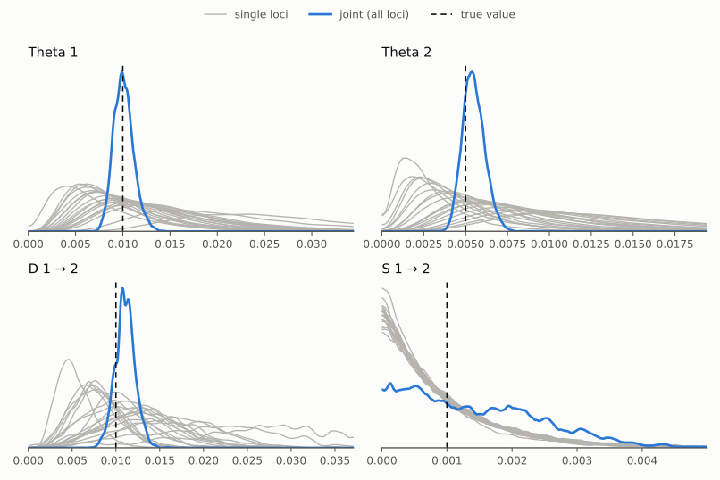
The figure (../00-basics/scripts/plot_posteriors.py bayesfile ...) shows
the difference between the two divergence parameters: every locus has an
opinion about D, and together they pin it down; for S the single loci
follow the prior (thin gray lines, falling from 0), and even the Joint
posterior only says that S is small.
The data-scaled prior also fits better: the marginal likelihood of
two-split rises from -18917.5 to -18888.5 (BTI), 29 log units.
4. Two populations: split, split with gene flow, or gene flow only?
Three models for two.txt, the marginal likelihoods from the BTI column
(sum over loci, “All … (independent parameters)”):
| Model | Prior | log ML (BTI) | Difference to best | Estimates |
|---|---|---|---|---|
| two-split (true) | gamma | -18888.5 | 0 | D 0.0111, S 0.0013 |
| two-splitmig | gamma | -18931.9 | -43.4 | M_1->2 5.0 (0-19), D 0.0116 |
| two-split (true) | default | -18917.5 | -29.0 | D 0.0119, S 0.0030 |
| two-splitmig | default | -18952.2 | -63.7 | M_1->2 4.3 (0-18), D 0.0122 |
| two-mig | default | -19001.7 | -113.2 | M_2->1 3.0 (0-16), M_1->2 47 (20-73) |
- The split without gene flow wins with either prior.
- The model with gene flow after the split finds M_1->2 near zero; the data give no reason for the extra parameter.
- The model with gene flow but no split is far behind. It explains the shared ancestry of Bute and Arran as migration into Bute (4Nm = Theta_2 x M_1->2, about 0.23 here), a different history that fits the data worse.
The two split models are nested (M_1->2 = 0 gives two-split), and the
difference between nested models is small in truth: with 16 heated chains it
shrinks to 2-6 log units. Five chains choose the right model, but use a
longer ladder (for example heating=YES:1:POWER:16) when the size of a Bayes
factor matters.
5. Three populations: which population tree?
Two trees for three.txt: the true chain (Coll split from Bute, Bute from
Arran) and a star (Bute and Coll both split from Arran):
| Prior | three-chain (true), log ML (BTI) | three-star, log ML (BTI) | Difference |
|---|---|---|---|
| gamma | -21429.3 | -21514.9 | -85.6 |
| default | -21515.6 | -21599.5 | -83.9 |
The true tree wins by more than 80 log units with either prior. The Joint medians of the chain model (true values next to the names, 95% HPD intervals for the split times):
| Parameter | Default prior | Gamma prior |
|---|---|---|
| Theta_1 (0.01) | 0.0094 | 0.0094* |
| Theta_2 (0.01) | 0.0087 | 0.0090* |
| Theta_3 (0.005) | 0.0068 | 0.0064* |
| D_1->2 (0.01) | 0.0118* (0.0097-0.0139) | 0.0108* (0.0097-0.0122) |
| S_1->2 (0.001) | 0.0023* | 0.0005* |
| D_2->3 (0.003) | 0.0048* (0.0037-0.0057) | 0.0041* (0.0035-0.0048) |
| S_2->3 (0.0005) | 0.0010* | 0.0009* |
The old split is estimated well. The recent split of Coll comes out older than in truth (0.0041-0.0048 against 0.003), and Theta_3 larger: few lineages of Coll coalesce before they join Bute, so the data say little about the time of the recent split. The interval does not cover the truth in this data set; section 6 repeats the analysis on 20 data sets.
With seven parameters most Joint rows carry the star (reweighting ESS 35-76):
the genealogy-sampling error of the Joint estimate is large (01-migration,
section 4). Longer runs or replicates with joint-samples reduce it
(01-migration, section 8).
In the star model both splits move to 0.0054-0.0062, between the two true times; a wrong tree gives misleading split times, so compare trees before reading the times.
6. How good are the split estimates? Twenty data sets
One data set cannot tell chance from bias. study/coverage_simulate.py
simulates many data sets with the truth of three.txt (the same simulator
as scripts/simulate_divergence.py), and study/coverage_summary.py
counts, for each parameter, how often the 95% HPD interval of the Joint
estimate covers the truth and how far the medians are from it:
python3 study/coverage_simulate.py study/coverage 20      # study/coverage/rep000 ... rep019
# run the three-chain model on each data set, one directory per run:
#   study/coverage/runs/SETTING/repNNN/outfile
python3 study/coverage_summary.py study/coverage
The three-chain model was run on 20 data sets with three prior settings (POWER:5 heating, 10000 samples, migrate-n 7.0.104; about 4.5 min per run on 21 MPI processes of a cluster):
- default: D uniform 0-0.1, S exponential with mean 0.1;
- gamma: the data-scaled priors of section 3, the same for both splits (D gamma with mean 0.01, S exponential with mean 0.001);
- gamma per split: as gamma, but the recent split gets its own D prior with mean 0.004:
bayes-priors= SPLIT * * GAMMAPRIOR: 0.0 0.01 0.05 2.0
bayes-priors= SPLIT 2 3 GAMMAPRIOR: 0.0 0.004 0.05 2.0
The second line overrides the first for the split 2->3 (Coll from Bute). Its mean comes from the data, not from the truth: the rough estimate D = (d_xy - pi_parent) / 2, with d_xy the average difference per site between Bute and Coll and pi_parent the diversity of Bute, gives 0.0016-0.0046 across the 20 data sets (and 0.0083-0.0130 for the old split).
Coverage of the 95% HPD intervals (out of 20) and median divided by the truth (mean over the data sets):
| Parameter (true) | default | gamma | gamma per split |
|---|---|---|---|
| D_1->2 (0.01) | 15, 1.14 | 18, 1.04 | 18, 1.02 |
| S_1->2 (0.001) | 13, 2.33 | 20, 1.10 | 20, 1.24 |
| D_2->3 (0.003) | 15, 1.19 | 17, 1.15 | 18, 1.06 |
| S_2->3 (0.0005) | 19, 1.53 | 13, 1.79 | 20, 1.13 |
| Theta_1 (0.01) | 17, 0.95 | 17, 0.97 | 19, 0.98 |
| Theta_2 (0.01) | 20, 1.03 | 20, 1.04 | 20, 1.04 |
| Theta_3 (0.005) | 20, 0.99 | 20, 1.03 | 19, 1.05 |
- The recent split comes out too old on average, by 19% with the default prior and 15% with one gamma prior for both splits. The data set of section 5 (1.6 and 1.4 times the truth) is at the upper end of this range.
- Most of the bias comes from the prior. A prior with mean 0.01 pulls the recent split toward 0.01, and the data say little about it (section 5). With its own prior at the scale of the data, the recent split is off by 6% and its interval covers the truth in 18 of 20 data sets.
- The spread S follows the same pattern: with the default prior (mean 0.1, a hundred times the truth) S_1->2 is more than twice too large; the per-split prior also brings S_2->3 to the truth, although its own prior did not change. D and S of one split are estimated together; a likely reason is that a split placed too old needs a wider spread to fit the lineages that left early (not tested here).
- The Thetas are fine with every prior.
- Most Joint rows are starred in every setting (reweighting ESS below 50 or a large bootstrap error); the medians and coverages above are nevertheless close to their targets. With seven parameters the Joint combination needs longer runs for clean rows (01-migration, section 8).
Advice: to compare population trees (section 5), keep the same priors for every split, so that the models differ only in the tree. To estimate the split times in the chosen tree, give each split its own D prior, with a mean from a rough estimate such as (d_xy - pi_parent) / 2, and an S prior at about a tenth of that mean.
7. Ordering the splits: divergence-order
In a chain 1 |-> 2 |-> 3, population 3 splits from population 2, which
itself exists only after it split from population 1. Forward in time, the
split 1->2 must come before the split 2->3; backward in time (lineage view),
D_1->2 must be larger than D_2->3. Nothing in the split model itself forces
this: the two mean split times are separate parameters. The option
divergence-order sets the constraint (TREE and NONE since 7.0.105 / 6.1.81,
RANK since 7.0.106 / 6.1.82):
divergence-order=TREE                     # default: the order the tree implies
divergence-order=NONE                     # no constraint
divergence-order=RANK: 1->2 2->3 1->4     # every split, oldest first
TREEkeeps a split older than the split that created its parent population. Splits from the same parent (sisters, for example 1->2 and 1->4 from a mainland 1) stay free with respect to each other.RANKlists every split of the model, oldest first; the mean split times then follow exactly this order, sisters included. Migrate stops with a message when a split is missing or listed twice, when the list contradicts the tree (2->3 before 1->2 above), or when tied splits (t) are not next to each other.NONEis the behaviour of migrate before 7.0.105; the runs of sections 3-6 (7.0.104) are unordered.
The constraint applies to the mean split times D in the per-locus chains and in the Joint combination. The split times of single lineages, drawn from Normal(D, S), may still cross.
When does it matter? study/coverage_simulate.py with the scenario close
simulates two close splits, D_1->2 = 0.006 and D_2->3 = 0.004 (S 0.0005
each, other values as in three.txt):
python3 study/coverage_simulate.py study/close 20 close
The three-chain model with the gamma priors of section 3 (the same prior for both splits) on 20 such data sets, without and with the order (NONE: 7.0.104; TREE: 7.0.106; about 5 min per run on 21 MPI processes):
| Parameter (true) | NONE: covered, median/true (sd) | TREE: covered, median/true (sd) |
|---|---|---|
| D_1->2 (0.006) | 18, 1.06 (0.07) | 16, 1.10 (0.10) |
| S_1->2 (0.0005) | 14, 1.84 (0.60) | 17, 1.98 (0.70) |
| D_2->3 (0.004) | 19, 1.03 (0.11) | 20, 1.02 (0.06) |
| S_2->3 (0.0005) | 15, 1.66 (0.71) | 19, 1.39 (0.38) |
| Theta_1 (0.01) | 20, 0.99 | 17, 0.99 |
| Theta_2 (0.01) | 17, 1.03 | 17, 1.04 |
| Theta_3 (0.005) | 20, 0.95 | 20, 0.96 |
- Without the order, the Joint medians of all 20 data sets are in the right order anyway; in 6 of them the two intervals overlap (2 with the order). With 20 loci the data order these splits on their own.
- The order sharpens the recent split: the spread of its medians across the data sets halves (sd 0.11 to 0.06), and S_2->3 is less inflated.
- The older split moves up a little (median 1.06 to 1.10 times the truth, covered in 16 instead of 18 data sets): here the constraint moved the older split up rather than the younger one down. The gamma prior with mean 0.01 pulls in the same direction.
- S_1->2 stays too large with either setting (1.8-2.0 times the truth): its prior (mean 0.001) is twice the true value, and the data say little about it. A plan to express the S prior relative to D is in docs/split_std_cv_plan.md.
Keep the default TREE. Use RANK only when there is independent evidence
for the order of sister splits (geology, fossils); otherwise leave sister
splits free and let the data decide.
8. Ancient samples: tip dates
When some samples are old (ancient DNA, museum specimens, virus isolates from different years), their lineages start in the past, not at the present. Migrate places each sample at its own age when it gets a file with the sampling dates.
data/dated.txt (scripts/simulate_tipdates.py) has the history of
three.txt (section 1, the same true values), but five of the ten Arran
sequences are ancient: Arr05-Arr09 were sampled 10,000, 20,000, 30,000,
40,000 and 50,000 years ago. The simulation uses 20 years per generation and
a mutation rate of 2e-6 per site and generation, so 10,000 years are 500
generations or 0.001 on the mutation scale; the oldest sample is 0.005 old,
half a Theta_1 and half the old split time.
The data show the ages. The ancient sequences differ less from Bute than the modern ones (per site: 0.030 for the modern Arran samples, 0.024 for the oldest), because their lineages had less time to collect mutations; a pair of a modern and an ancient Arran sequence differs more than a modern pair (0.0115 against 0.0082), because the two lineages can only coalesce before the age of the ancient one.
The date file, data/dated.dates, has a title line, then for each
population a line with the number of samples and the name, and one line per
sample: the name in the first 10 columns (the name length of the infile),
then the age:
dated.txt: sampling ages in years before present
10 Arran
Arr00     0
...
Arr05     10000
...
Arr09     50000
10 Bute
But00     0
...
Migrate finds the dates by the sample names, so the names must match the
infile. Lines starting with # are skipped. The ages count backward from the
present (lineage view), and the youngest sample marks the present. A title
line starting with F switches to forward dates (calendar years); do not
start a title with F by accident, and use ages before present.
Three parmfile lines turn the ages into mutation-scale times (age x generations per year x mutation rate per generation):
tipdate-file=YES:dated.dates
generation-per-year=0.05
mutationrate-per-generation={2e-6}
generation-per-year is the inverse of the generation time (here 20
years). The mutation rate is per site and generation for DNA; give one value
per locus, or one value for all. The models (scripts/make_parmfiles.sh):
dated-tips is the true chain model with the gamma priors of section 3
(parmfile.three-chain-gamma) and the date file, dated-notips the same
model on the same data without the date file, as if all samples were modern.
Joint medians and 95% HPD intervals (POWER:5; with tip dates 7.0.108 on 6 MPI processes, 8 min; without tip dates 7.0.106 on 11 MPI processes, about an hour on a busy machine):
| Parameter (true) | With tip dates | Without tip dates |
|---|---|---|
| Theta_1 (0.01) | 0.0086 (0.0071-0.0103) | 0.0139* (0.0114-0.0165) |
| Theta_2 (0.01) | 0.0108 (0.0087-0.0128) | 0.0117* (0.0095-0.0141) |
| Theta_3 (0.005) | 0.0047* (0.0034-0.0061) | 0.0045* (0.0034-0.0057) |
| D_1->2 (0.01) | 0.0107* (0.0096-0.0117) | 0.0109* (0.0085-0.0120) |
| S_1->2 (0.001) | 0.0012* (0.0002-0.0023) | 0.0004* (0.0001-0.0032) |
| D_2->3 (0.003) | 0.0038* (0.0028-0.0045) | 0.0038* (0.0025-0.0051) |
| S_2->3 (0.0005) | 0.0010* (0.0001-0.0021) | 0.0012* (0.0002-0.0021) |
| log ML (BTI, joint) | -21790.5 | -21905.4 |
- The dates matter most for Arran, the population with the ancient samples: Theta_1 is 0.0086 with the dates (the interval covers 0.01) and 0.0139 without them (the interval misses 0.01).
- The split times change little: both intervals of D_1->2 and D_2->3 cover the true values.
- The marginal likelihood prefers the dates by 115 log units: the right sampling times fit the data much better than treating all samples as modern.
Before Migrate 7.0.108 and 6.1.84, MPI runs used the sampling dates only for the first locus when the infile has all loci of an individual on one line (as here); the other loci were analysed as if all samples were modern. Serial runs were not affected. An earlier version of this section showed such an MPI run: its estimates and marginal likelihood (-21903.5) were almost those without dates.
To check that Migrate uses the dates, print the genealogies
(print-tree=LASTCHAIN:1:treefile in a short run) and look at every locus,
not only the first: the ancient tips end above the present, Arr09 0.002 above
Arr07 (50,000 against 30,000 years). tools/check_tipdate_trees.py (in the
repository) does this for all loci.
9. What next
- 03-growth: populations that grow or shrink, and how to test for growth.
- The divergence model with migration after the split (
D) and with population trees of more than three populations follows the same steps: the same priors for every split when comparing trees, a prior per split when estimating the split times.