03 Growth: populations that grow or shrink
Draft: work in progress. This recipe is not finished yet; sections may be incomplete and results may change.
Status: draft (2026-11-11), sections 1-9. Run with migrate-n 7.0.106 and 7.0.107 (they differ only in the tip-date and heating options, which these runs do not use differently).
This recipe estimates exponential growth. It uses simulated data sets: one population that grows, one at constant size, one that shrinks, and two populations of which one grows. It shows how to switch growth on, how to read the growth rate, why its estimate is biased upward and how more loci fix that, how to test whether a population grows at all, and applies this to a real mitochondrial data set of a frog. Read 00-basics and 01-migration first.
Contents
- The data and the true values
- Growth in the parmfile
- The growth rate and its prior
- One growing population
- Constant size or growth?
- A shrinking population
- Two populations, one growing
- A real data set: the pool frog
- What next
1. The data and the true values
All data sets have 20 DNA loci of 500 bp and 20 sequences per population,
simulated with msprime under the Jukes-Cantor model
(scripts/simulate_growth.py; truth in data/truth.txt).
| Data | Population(s) | Theta (today) | Growth g | Migration |
|---|---|---|---|---|
grow.txt | Arran | 0.01 | 200 | - |
const.txt | Arran | 0.01 | 0 | - |
shrink.txt | Arran | 0.01 | -50 | - |
twopop.txt | Arran, Bute | 0.01, 0.005 | 200, 0 | M_2->1 = 100, M_1->2 = 400 |
2. Growth in the parmfile
Migrate uses the exponential model of Kuhner, Yamato & Felsenstein (1998). Backward in time (lineage view), Theta at time t before the present is
Theta(t) = Theta exp(-g t)
Theta is today’s value, and t is on the mutation scale (generations times the mutation rate), like the divergence times of 02-divergence. A positive g means that the population grows forward in time (it was smaller in the past); a negative g means that it shrinks forward in time (it was larger in the past). The growth rate per generation is g times the mutation rate per generation; for these data (1e-7 per site) g = 200 is 2e-5 per generation.
A useful scale: the genealogy of a sample reaches back about Theta on the
same time scale, so g x Theta is the number of e-fold changes over the depth
of the genealogy. For grow.txt, 200 x 0.01 = 2: Theta at the root of a
typical genealogy is about exp(-2) = 0.14 of today’s value.
One line switches growth on, one number per population:
| population-growth | Meaning |
|---|---|
{0} | all populations constant (the default) |
{1} | all populations grow with the same rate Growth_1 |
{1 0} | population 1 grows (Growth_1), population 2 is constant |
{1 2} | each population has its own rate, Growth_1 and Growth_2 |
{1 0 1} | populations 1 and 3 share one rate, population 2 is constant |
The models of this recipe (scripts/make_parmfiles.sh writes them; they
differ only in the data file and population-growth):
| Model | Data | population-growth |
|---|---|---|
| grow-const, grow-growth | grow.txt | {0}, {1} |
| const-const, const-growth | const.txt | {0}, {1} |
| shrink-const, shrink-growth | shrink.txt | {0}, {1} |
| twopop-const, twopop-arran, twopop-both | twopop.txt | {0}, {1 0}, {1 2} |
| lessonae-const, lessonae-growth (section 8) | lessonae56.txt | {0}, {1} |
Run one model with scripts/run.sh MODEL BINARY RUNDIR [NPROC], for example
scripts/run.sh grow-growth migrate-n-mpi runs/grow-growth 6
All runs use the settings of 01-migration (10000 samples, long-inc 100,
burn-in 10000 samples) with heating=YES:1:POWER:5. On 6 MPI processes of a
laptop a one-population model takes 2-3 min, a two-population model 15-40 min.
3. The growth rate and its prior
The growth rate is the parameter Growth_1 (Growth_2, …) in the outfile.
Without a bayes-priors line Migrate uses a uniform prior from -1000 to 1000
(the outfile lists it under “Population growth”). The parmfile written by
Migrate does not show this default; to change it, add a line such as
bayes-priors= GROWTH * * UNIFORMPRIOR: -100.0 1000.0 100.0
(UNIFORMPRIOR: min max delta; delta is the width of the proposal window.)
The default is wide on purpose, but its negative half is a problem. With g x Theta = -10 (g = -1000, Theta = 0.01) the population was e^10 times larger at the depth of a typical genealogy, and two lineages may never meet: for g < 0 the coalescent is defective, the time to the common ancestor is infinite with positive probability. Section 5 shows that a prior reaching that far changes the marginal likelihood of the growth model.
4. One growing population
grow.txt (true Theta 0.01, g 200), Joint rows:
| Model | Theta_1 | 95% HPD | Growth_1 | 95% HPD |
|---|---|---|---|---|
| grow-growth | 0.0134 | 0.0094-0.0179 | 487 | 255-740 |
| grow-const | 0.0076 | 0.0062-0.0091 | - | - |
- The growth model finds growth, but g is 2.4 times the truth and its interval misses it; Theta is a third too large.
- The constant model averages Theta over the depth of the genealogy and reports a value below today’s Theta.
Is that a bias or bad luck? study/simulate_replicates.py simulates more
data sets with the truth of grow.txt, and study/summary.py counts how often
the 95% HPD interval of the Joint estimate covers the truth:
python3 study/simulate_replicates.py study/L20 20     # study/L20/rep00 ... rep09
# run grow-growth in each repNN directory, then
python3 study/summary.py study/L05 study/L20 study/L50
grow-growth on 10 data sets each, with 5, 20 and 50 loci (default prior, POWER:5):
| Loci | g: HPD covers truth | g: median / truth | g: HPD width | Theta: covers | Theta: median / truth |
|---|---|---|---|---|---|
| 5 | 7/10 | 1.67 | 626 | 10/10 | 1.20 |
| 20 | 10/10 | 1.38 | 342 | 10/10 | 1.07 |
| 50 | 10/10 | 0.99 | 181 | 10/10 | 1.02 |
(median over the 10 data sets of the posterior median divided by the truth, and the median width of the 95% HPD interval)
- With 20 loci the intervals cover the truth, but the estimates of g are skewed upward; grow.txt (487) is above all ten replicates (185-326), an unlucky data set rather than the typical case.
- With 5 loci g is 1.7 times the truth, and the three intervals that miss all lie above it. With 50 loci the bias is gone.
- Theta follows g: the two are correlated, and a too-large g comes with a too-large Theta.
Kuhner, Yamato & Felsenstein (1998, Genetics 149: 429-434) found the same upward bias with maximum likelihood (FLUCTUATE), and named two causes, both part of estimating growth from genealogies, not of the sampler:
- g depends nonlinearly on the coalescence times, so the random spread of these times turns into an upward bias.
- Every genealogy ends at its last coalescence. The coalescent distribution is cut there, which makes a population that was small near the root (a bottleneck) an attractive explanation. Even a genealogy with exactly the expected interval lengths gives a positive estimate.
They also note that genealogies with infinite time (possible for g < 0) are excluded, which adds an upward bias they expected to be trivial. Their remedy is the one in the table: more unlinked loci, which help far more than more sequences or longer loci. For a sample of two sequences and true g = 0 their mean estimate fell from 20.3 with one locus to 1.3 with three loci and 0.02 with 100 loci. With few loci, read a positive g as an upper estimate.
5. Constant size or growth?
The marginal likelihoods (BTI column, sum over loci, “All … (joint)”) of the constant and the growth model for the three one-population data sets (default prior, POWER:5):
| Data (true g) | constant | growth | growth - constant | Growth_1 (95% HPD) |
|---|---|---|---|---|
| grow.txt (200) | -16440.5 | -16397.6 | +42.9 | 487 (255-740) |
| const.txt (0) | -17308.4 | -17284.2 | +24.2 | -12.7 (-61-35) |
| shrink.txt (-50) | -17938.9 | -17916.2 | +22.7 | -35 (-71–4) |
The growth model wins for const.txt by 24 log units, although its estimate (-12.7, interval across 0) says that there is no growth. Two things inflate the growth model here.
The ladder. With 16 heated chains (heating=YES:1:POWER:16) the difference
for const.txt drops to +10.6 (and +23.7 for grow.txt). Five chains are fine
for choosing between models with a clear margin, but this margin is not
clear.
The prior. The same runs with 16 chains and a growth prior that does not reach far below 0:
| Growth prior | const.txt: growth - constant | grow.txt: growth - constant |
|---|---|---|
| -1000 to 1000 (default) | +10.6 | +23.7 |
| -100 to 1000 | +0.2 | +13.6 |
| 0 to 1000 | -2.8 | +12.6 |
With a prior from -100 or 0, constant size and growth tie for const.txt or the constant model wins, as they should; grow.txt still prefers growth by 13 log units. A wider prior should lower the marginal likelihood of the growth model a little, not raise it: going from -100 to -1000 widens it by a factor 1.8, which costs about 0.6 log units. The rise of about 10 log units for both data sets comes from the strongly negative growth rates, where the coalescent is defective (section 3); we have not traced the mechanism in the heated chains. These are single runs.
With five chains (POWER:5) the narrower prior removes about 11 log units in all three data sets, but the ladder effect remains:
| Data (true g) | growth - constant, prior -1000 to 1000 | growth - constant, prior -100 to 1000 | Growth_1 (95% HPD), -100 to 1000 |
|---|---|---|---|
| grow.txt (200) | +42.9 | +31.5 | 513 (292-768) |
| const.txt (0) | +24.2 | +12.5 | -15.3 (-67-32) |
| shrink.txt (-50) | +22.7 | +12.0 | -34 (-69–4) |
With five chains const.txt still prefers growth by 12 log units; the estimate of g, with its interval across 0, is the better guide there.
Advice: to test for growth, use a growth prior whose lower bound stays within a few e-folds over the depth of the genealogy, g > -2/Theta or so (-200 for Theta = 0.01), or at 0 if decline is not a question. The narrower prior also gives better estimates when a population has no growth to find (section 7). Use a longer ladder when the difference is less than about 20 log units, and read the estimate of g next to the Bayes factor.
6. A shrinking population
shrink.txt (true Theta 0.01, g -50):
| Model | Theta_1 | 95% HPD | Growth_1 | 95% HPD |
|---|---|---|---|---|
| shrink-growth | 0.0098 | 0.0080-0.0117 | -35 | -71 to -4 |
| shrink-const | 0.0112 | 0.0093-0.0129 | - | - |
The growth model finds the decline (g < 0, interval below 0) and today’s Theta. The constant model again reports Theta averaged over the depth of the genealogy, here larger than today’s value because the population was larger in the past. A decline with g x Theta = -0.5 is mild; a prior with lower bound -100 (section 5) contains it.
7. Two populations, one growing
twopop.txt: Arran grows (g 200), Bute is constant, with migration in both directions (M_2->1 = 100, M_1->2 = 400). Joint rows (* = the Joint estimate has a large genealogy-sampling error, 01-migration section 8):
| Model | log ML (BTI) | Theta_1 | Theta_2 | M_2->1 | M_1->2 | Growth_1 | Growth_2 |
|---|---|---|---|---|---|---|---|
| truth | 0.01 | 0.005 | 100 | 400 | 200 | 0 | |
twopop-const {0} | -19419.3 | 0.0080* | 0.0035 | 92* | 702 | - | - |
twopop-arran {1 0} | -19410.5 | 0.0090 | 0.0036 | 154* | 656* | 102* (11-267) | - |
twopop-both {1 2} | -19395.7 | 0.0092* | 0.0032* | 126* | 595* | 125* (4-328) | -665* (-1000 to -111) |
- The true model (
{1 0}) finds growth in Arran, with an interval that covers 200. - The model with a separate rate for Bute wins by 15 log units, but its Growth_2 piles up at the lower bound of the prior (-1000). This is the defective region of section 5 again, not evidence of a decline.
- All models underestimate Theta_2 (0.0032-0.0036 instead of 0.005) and overestimate M_1->2 (600-700 instead of 400); their product 4Nm_1->2 = Theta_2 x M_1->2 (about 2.2-2.5, truth 2.0) is better determined than its two factors (01-migration).
- Most two-population rows are starred; the Joint combination of six parameters needs longer runs.
The same models with the growth prior -100 to 1000 (POWER:5):
| Model | log ML (BTI) | Theta_1 | Theta_2 | M_2->1 | M_1->2 | Growth_1 | Growth_2 |
|---|---|---|---|---|---|---|---|
twopop-arran {1 0} | -19403.9 | 0.0088 | 0.0044 | 218 | 442 | 177 (44-329) | - |
twopop-both {1 2} | -19399.9 | 0.0096 | 0.0044 | 165* | 546* | 125* (-2-276) | 105* (-100-620) |
- With this prior the true model has no starred rows, and all its estimates are close to the truth: g 177 with an interval around 200, Theta_2 and M_1->2 near their true values.
- twopop-both still wins, now by 4 log units, again with Growth_2 at the lower bound of its prior (mode -99). Two nested models 4 log units apart with five chains are not a clear decision (section 5); the estimate of Growth_2, with an interval from the bound to 620, says that Bute’s growth is not determined.
8. A real data set: the pool frog
The pool frog Pelophylax lessonae now has a large range in Europe; during the last glaciation it was probably restricted to a few refugia in the south. Does its mitochondrial DNA show the expansion?
The data: ND2 (1038 bp) and ND3 (340 bp) of 56 frogs with lessonae
mitochondria, from Ploetner et al. (2008, J Evol Biol 21: 668-681), GenBank
AM749714-AM749730 and AM887938-AM887976. scripts/fetch_lessonae.py
downloads them and writes data/lessonae56.txt and the sample list
data/lessonae56.tsv. Some carriers are hybrids (P. esculentus) or
P. ridibundus with lessonae mitochondria; GenBank lists the frog’s
species, but all 56 sequences belong to the lessonae lineage. Most come
from the north of the range (Sweden 27, Germany 14, Baltic states and
Poland 8, Denmark 2), few from the south (Italy 2, Romania 2, Slovakia 1).
There are 24 variable sites and 17 haplotypes in three clusters: L1-L12
(49 sequences, star-shaped around L2, all over the north and one in the
Danube delta), L13 (Carbonare, Italy), and L14-L17 (Danube delta, Slovakia,
Poland, Schleswig-Holstein).
One locus, so no inheritance scalar is needed: Theta is the Theta of this
mitochondrial locus. The parmfiles (parmfile.lessonae-const,
parmfile.lessonae-growth) use F84 with base frequencies from the data,
50000 samples and 16 heated chains (heating=YES:1:POWER:16). The growth
model has the prior
bayes-priors= GROWTH * * UNIFORMPRIOR: -500.0 10000.0 1000.0
because the default (-1000 to 1000) and also an upper bound of 5000 cut off the posterior. A run takes about 10 min on one core.
| Model | Theta_1 (95% HPD) | Growth_1 (95% HPD) | log ML (BTI) | Difference |
|---|---|---|---|---|
| constant | 0.0048 (0.0027-0.0085) | - | -2146.16 | 0 |
| growth | 0.0089 (0.0032-0.0377) | 1548 (11-6059) | -2144.38 | +1.8 |
(outfile modes of the marginal posteriors.) The growth model is better by 1.8 log units, a posterior probability of about 0.86 with equal prior probabilities: positive, but weak evidence. The growth rate is positive (P(g > 0) = 0.995), but its interval spans a factor of 500.
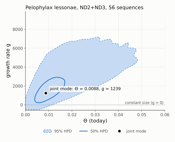
The figure (scripts/plot_theta_growth.py bayesallfile OUT.svg --prior -500 10000 --theta-max 0.06; --tagged-pdf also writes a tagged PDF/UA-2 version
with alt text) shows why: the data do not fix Theta and g separately. The 95%
region is a ridge from small Theta with slow growth to large Theta with fast
growth; what the single locus determines is Theta some time back, and that
the population grew since then.
The modes need care in a posterior like this. The figure marks the joint mode of the two-dimensional density (Theta 0.0088, g 1239); the outfile reports the modes of the two marginal distributions (0.0089, 1548). On a tilted ridge that widens toward large g, integrating Theta out moves the mode of g up; on a log axis for Theta the mode would move again (the density of log Theta is Theta p(Theta)). When the marginal is flat, as for Theta here, its mode depends on the bins and the smoothing. Report medians and HPD intervals, and call a mode in a two-dimensional figure the joint mode.
Two cautions. First, a single locus: section 4 showed that one locus overestimates g, so read g as an upper estimate. Second, the model assumes one population. The sample mixes the star-shaped northern cluster with the older southern clusters. Cluster L1-L12 alone (49 sequences, a subset chosen by the genealogy, for illustration only) prefers growth by 5.1 log units, and its g piles up at the upper bound of the 5000 prior. The deep clusters dilute the expansion signal of the north. Testing whether they come from separate refugia needs populations defined by geography and nuclear loci, not the mitochondrial clusters themselves (which would be circular).
9. What next
- 04-skyline: population sizes through time without assuming exponential growth (event-histogram skylines and skyline=PARAM).
- 05-model-selection: marginal likelihoods, heating ladders and Bayes factors in more detail; section 5 of this recipe is one reason to read it.