04 Skyline: population sizes and migration rates through time
Draft: work in progress. This recipe is not finished yet; sections may be incomplete and results may change.
Status: draft (2026-11-11), sections 1-10. Run with migrate-n 7.0.110 (the empirical skylines with 7.0.109, which computes them the same way); sections 4 and 6 checked with 6.1.86.
This recipe estimates how Theta and M change through time. Migrate has two
skylines: an empirical one, read from the sampled genealogies of an ordinary
run, and a parametric one (skyline=PARAM), in which Theta or M get a
multiplier per time segment that is estimated with the other parameters.
The data are simulated: a constant population, one that expanded, one that
declined, the expansion with ancient samples (tip dates), and two
populations whose migration rate changed. Read 00-basics, 01-migration and
03-growth first; section 6 uses the tip dates of 02-divergence.
Contents
- The data and the true values
- Skylines in the parmfile
- The empirical skyline
- The parametric skyline
- Constant size or a change?
- Ancient samples: with and without the date file
- Cycles: how far back can a skyline see?
- Migration through time
- Both versions of Migrate
- What next
1. The data and the true values
All data sets have 20 DNA loci of 500 bp and 20 sequences per population,
simulated with msprime under the Jukes-Cantor model
(scripts/simulate_skyline.py; truth in data/truth.txt). Times are
backward from the present (lineage view) on the mutation scale, like the
divergence times of 02-divergence; “before t” means older than t.
| Data | Population(s) | Today | Before the change | Change at t |
|---|---|---|---|---|
const.txt | Arran | Theta 0.01 | - | - |
expand.txt | Arran | Theta 0.01 | Theta 0.002 | 0.003 |
decline.txt | Arran | Theta 0.01 | Theta 0.05 | 0.002 |
dated.txt | Arran, 10 of 20 samples ancient | Theta 0.01 | Theta 0.002 | 0.003 |
twopop.txt | Arran, Bute (Theta 0.01, 0.005; M_1->2 = 400) | M_2->1 = 100 | M_2->1 = 500 | 0.003 |
cyclic.txt, cyclic-dated.txt | Arran, 40 sequences | Theta(t) = 0.01 x 3^sin(2 pi t / 0.004) | three cycles | - |
Forward in time, expand.txt grew five-fold at t = 0.003, decline.txt
shrank five-fold at t = 0.002, and in twopop.txt immigration into Arran
from Bute dropped five-fold at t = 0.003. dated.txt has the history of
expand.txt, but ten samples are 5,000 to 50,000 years old
(data/dated.dates); with 20 years per generation and a mutation rate of
2e-6 per site and generation, 10,000 years are 0.001 on the mutation scale,
so the expansion happened 30,000 years ago and the ancient samples lie on
both sides of it. The cyclic data sets (section 7) have 40 sequences; Theta
swings between 0.0033 and 0.03 with a period of 0.004 (data/cyclic-truth.txt
has the steps of the simulation); in cyclic-dated.txt 20 of the 40
samples are 3,000 to 60,000 years old (t = 0.0003-0.006).
2. Skylines in the parmfile
The models of this recipe (scripts/make_parmfiles.sh writes them from
the parmfile Migrate writes itself; they differ only in the lines below):
| Model | Data | Skyline lines |
|---|---|---|
| const-yes, expand-yes, decline-yes, dated-yes, twopop-yes | as named | skyline=YES:0.0005:skylinefile |
| const-param, expand-param, dated-param, dated-nodates | as named | skyline=PARAM:2:0.0005:skylinefile, skyline-times={0.003} |
| decline-param | decline.txt | skyline=PARAM:2:0.0005:skylinefile, skyline-times={0.002} |
| expand-grid, decline-grid | as named | skyline=PARAM:5:0.0005:skylinefile, skyline-times={0.002 0.004 0.006 0.008} |
| twopop-mig | twopop.txt | as const-param, and skyline-model={c * c c} |
| cyclic-yes, cyclic-dated-yes | as named | skyline=YES:0.0005:skylinefile |
| cyclic-grid, cyclic-dated-grid | as named | skyline=PARAM:12:0.0005:skylinefile, skyline-times={0.001 0.002 ... 0.011} |
| cyclic-fine, cyclic-dated-fine | as named | skyline=PARAM:24:0.0005:skylinefile, skyline-times={0.0005 0.0010 ... 0.0115}, replicate=YES:3 (cyclic-dated-fine also joint-samples=1) |
Every model also has mig-histogram=ALL:0.0005:mighistfile: the skylines
need the event histograms. dated-yes and dated-param read the sampling
dates (section 6); dated-nodates is dated-param without them;
cyclic-dated-yes, cyclic-dated-grid and cyclic-dated-fine read
cyclic-dated.dates.
Run one model with scripts/run.sh MODEL BINARY RUNDIR [NPROC], for example
scripts/run.sh expand-param migrate-n-mpi runs/expand-param 5
The runs use the settings of 01-migration (10000 samples, long-inc 100,
burn-in 10000 samples) with heating=YES:1:POWER:5. On 5 MPI processes of
a laptop a one-population model takes 2-3.5 min (the cyclic 12-segment
models with 40 sequences 14-15 min; the 24-segment models with three
replicates ran on 59-61 MPI processes of a cluster, 14-16 min, and 34 min
with joint-samples=1), a two-population model 14-16 min.
The options:
skyline=YES:binsize:skylinefile        empirical skyline (section 3)
skyline=PARAM:n:binsize:skylinefile    parametric skyline with n segments (section 4)
skyline-times={t1 t2 ...}              segment boundaries (n - 1 values; they set n)
skyline-model={...}                    which parameters get multipliers (section 7)
bayes-priors= SKYLINE * * RANDOMWALK: sigma        prior of the multipliers (default sigma 1)
bayes-priors= SKYLINE * * LOGUNIFORM: min max      or independent log-uniform multipliers
mig-histogram and skyline share one bin size, the width of the time
bins of the empirical skyline. Without skyline-times, PARAM:n:width
makes n segments of that width, the last one open-ended; set the boundaries
with skyline-times and keep the small bin size, otherwise the empirical
skyline of the same run gets the coarse segment width as its bins.
3. The empirical skyline
Every run with skyline=YES (or PARAM) records, in time bins, how many
coalescences and migrations the sampled genealogies have and how long they
spent with how many lineages. In each bin it reports the value of a
parameter that is constant within the bin and fits these genealogies best
(maximum likelihood): the classic skyline of Pybus, Rambaut & Harvey (2000)
estimates Theta from each coalescent interval alone; grouping intervals, here
by time bin and over all sampled genealogies and loci, follows the
generalized skyline of Strimmer & Pybus (2001):
Theta = sum k(k-1) dt / number of coalescences in the bin
M     = number of migrations / sum k dt        (k lineages in the receiving population)
The error band is value / sqrt(coalescences per genealogy): the coalescent noise of one sample, large where few events happen (old bins). The skylinefile lists, per locus and for all loci (the last locus number), the bin age, value, events per genealogy, standard error, exposure per genealogy and number of events; the PDF plots it. Migrate before 7.0.109 averaged the per-interval estimates over the bin with time weights, which favours long intervals: on constant data its skyline was about twice Theta near the present and U-shaped.
Empirical skyline of Theta (all loci, median and the 95% band at the bin middle; truth in parentheses):
| t | const.txt (0.01) | expand.txt (0.01; 0.002 before 0.003) | decline.txt (0.01; 0.05 before 0.002) |
|---|---|---|---|
| 0.00025 | 0.0109 (0.0094-0.0126) | 0.0081 (0.0071-0.0092) | 0.0184 (0.0156-0.0218) |
| 0.00225 | 0.0113 (0.0068-0.0187) | 0.0075 (0.0043-0.0131) | 0.0190 (0.0118-0.0307) |
| 0.00425 | 0.0106 (0.0044-0.0255) | 0.0058 (0.0021-0.0158) | 0.0329 (0.0131-0.0830) |
| 0.00625 | 0.0090 (0.0026-0.0310) | 0.0053 (0.0010-0.0280) | 0.0445 (0.0123-0.1609) |
| 0.01025 | 0.0097 (0.0009-0.1076) | 0.0045 (0.0001-0.2586) | 0.0479 (0.0084-0.2735) |
The empirical skyline shows the direction and the rough timing of a change, but it smooths it and does not reach the old value: the genealogies come from a run that assumes a constant Theta, so they are drawn toward constant size. Use it to look, and the parametric skyline to estimate.
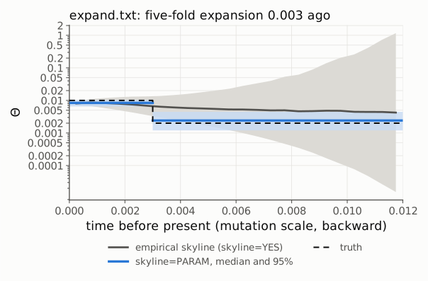
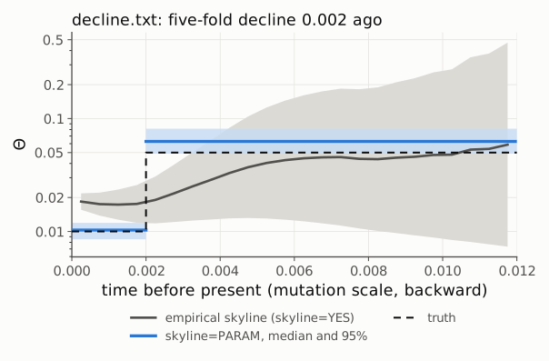
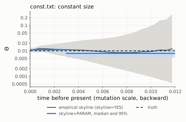
(scripts/plot_skyline.py: the grey line and band are the empirical
skyline, the blue lines and boxes the PARAM segments, the dashed line the
truth; log scale.)
4. The parametric skyline
With skyline=PARAM Theta (and M, section 7) gets a multiplier tau_s in
each segment s; the first segment is today (tau_1 = 1), so Theta is
today’s value and the value in segment s is Theta x tau_s. The prior of the
multipliers is a random walk on log tau (log tau_s - log tau_(s-1) normal
with standard deviation sigma = 1), or log-uniform. The outfile reports
the multipliers and the segment values (Joint median and 95% interval).
With the true boundary (two segments):
| Data | Theta today (true) | tau_2 (true) | Theta before the change (true) |
|---|---|---|---|
| const.txt | 0.0110 (0.0087-0.0132) (0.01) | 0.72 (0.46-1.13) (1) | 0.0079 (0.0055-0.0117) (0.01) |
| expand.txt | 0.0084 (0.0065-0.0103) (0.01) | 0.29 (0.14-0.56) (0.2) | 0.0024 (0.0012-0.0045) (0.002) |
| decline.txt | 0.0103 (0.0085-0.0119) (0.01) | 6.1 (4.4-8.5) (5) | 0.063 (0.049-0.081) (0.05) |
All intervals cover the truth. Without the skyline (the -yes runs, which
assume constant size) Theta is 0.0070 (0.0057-0.0082) for expand.txt and
0.0244 (0.0215-0.0276) for decline.txt: a constant-size model gives a
compromise between the sizes, and neither interval covers today’s value.
The boundary is rarely known. With five segments of width 0.002 (the last open-ended):
| Segment | expand.txt: Theta x tau (true) | decline.txt: Theta x tau (true) |
|---|---|---|
| today, 0-0.002 | 0.0088 (0.0067-0.0110) (0.01) | 0.0106 (0.0089-0.0126) (0.01) |
| 0.002-0.004 | 0.0030 (0.0017-0.0062) (0.01, 0.002 from 0.003) | 0.045 (0.022-0.123) (0.05) |
| 0.004-0.006 | 0.0032 (0.0010-0.0118) (0.002) | 0.062 (0.026-0.192) (0.05) |
| 0.006-0.008 | 0.0033 (0.0004-0.0179) (0.002) | 0.050 (0.019-0.199) (0.05) |
| before 0.008 | 0.0029 (0.0002-0.0263) (0.002) | 0.070 (0.051-0.098) (0.05) |
The grid finds the change and its size. Segments that hold few coalescences (here those after the bulk of the genealogy has coalesced, and the segment that contains the change) have wide intervals, and the random walk prior pulls neighbouring segments together; the open last segment collects everything older and is precise again.
5. Constant size or a change?
Marginal likelihoods (BTI, joint, POWER:5); the -yes model is the
constant-size model:
| Data | constant | PARAM, true boundary | PARAM, 5-segment grid | best minus constant |
|---|---|---|---|---|
| const.txt | -17382.5 | -17382.1 | - | +0.4 (tie) |
| expand.txt | -16302.4 | -16295.2 | -16292.1 | +10.3 |
| decline.txt | -22400.9 | -22341.1 | -22341.1 | +59.8 |
| dated.txt (section 6) | -16601.6 | -16561.1 | - | +40.5 |
The skyline wins clearly for the decline and the dated expansion, by 10 log units for the expansion without ancient samples, and ties for constant size; there the multiplier (0.72, interval across 1) also says “no change”. The grid does as well as the true boundary, so the boundary need not be known to detect a change. These are single runs with five heated chains; 03-growth (section 5) shows how the ladder and the prior move such numbers when the difference is small.
6. Ancient samples: with and without the date file
dated.txt is the expansion of section 4 with ten ancient samples. The date
file and the three parmfile lines are those of 02-divergence (section 8):
tipdate-file=YES:dated.dates
generation-per-year=0.05
mutationrate-per-generation={2e-6}
dated-param uses them, dated-nodates is the same model without them (as
if all samples were modern):
| Model | Theta today (0.01) | tau_2 (0.2) | Theta before 30,000 years (0.002) | log ML (BTI) |
|---|---|---|---|---|
| dated-param | 0.0106 (0.0079-0.0133) | 0.17 (0.12-0.25) | 0.0018 (0.0013-0.0024) | -16561.1 |
| dated-nodates | 0.0172 (0.0131-0.0209) | 0.048 (0.024-0.095) | 0.0008 (0.0004-0.0016) | -16733.0 |
With the dates every interval covers the truth, and the old segment is more precise than in section 4 without ancient samples (0.0013-0.0024 against 0.0012-0.0045): the ancient samples are lineages that start in the old segment. Without the dates Theta today is too high and the old Theta too low, and the marginal likelihood is 172 log units worse.
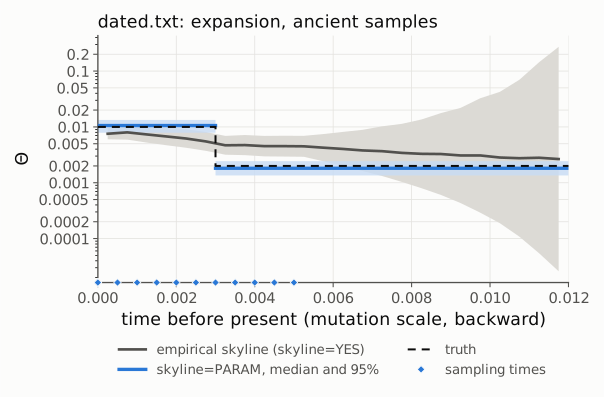
The small blue diamonds on the time axis mark the sampling times (plot_skyline.py --dates). The empirical skyline of dated-yes (constant Theta, with the dates) comes
closer to the truth than for expand.txt (0.0045 at t = 0.0043, 0.0028 at
0.0103), because the ancient samples add lineages in the old bins. Before
Migrate 7.0.108 and 6.1.84, MPI runs used the dates only for the first
locus of a data set like this one (02-divergence, section 8).
7. Cycles: how far back can a skyline see?
Real populations rarely change once. cyclic.txt has three cycles of
Theta between 0.0033 and 0.03 over t = 0-0.012; the parametric skyline uses
twelve segments of width 0.001 (the last open-ended), half a cycle each,
and 40 sequences. True value (geometric mean of Theta over the segment) and
the Joint estimates of the segment values:
| Segment | true | cyclic.txt (modern samples) | cyclic-dated.txt (half ancient) |
|---|---|---|---|
| 0-0.001 (today) | 0.020 | 0.017 (0.014-0.020) | 0.013 (0.010-0.016) |
| 0.001-0.002 | 0.020 | 0.020 (0.010-0.047) | 0.016 (0.010-0.026) |
| 0.002-0.003 | 0.005 | 0.0055 (0.0029-0.0136) | 0.0044 (0.0032-0.0062) |
| 0.003-0.004 | 0.005 | 0.0050 (0.0023-0.0181) | 0.0047 (0.0033-0.0072) |
| 0.004-0.005 | 0.020 | 0.0075 (0.0027-0.0276) | 0.019 (0.011-0.040) |
| 0.005-0.006 | 0.020 | 0.0061 (0.0017-0.0310) | 0.018 (0.009-0.041) |
| 0.006-0.007 | 0.005 | 0.0047 (0.0014-0.0229) | 0.0057 (0.0039-0.0099) |
| 0.007-0.008 | 0.005 | 0.0038 (0.0011-0.0207) | 0.0083 (0.0039-0.0262) |
| 0.008-0.009 | 0.020 | 0.0046 (0.0010-0.0288) | 0.0099 (0.0037-0.0360) |
| 0.009-0.010 | 0.020 | 0.0053 (0.0008-0.0400) | 0.0075 (0.0029-0.0300) |
| 0.010-0.011 | 0.005 | 0.0053 (0.0004-0.0560) | 0.0057 (0.0021-0.0218) |
| before 0.011 | 0.005-0.02 | 0.0051 (0.0002-0.0627) | 0.0082 (0.0040-0.0184) |
With modern samples only the first cycle is recovered; after t = 0.004 the estimates sit near the prior’s middle with intervals 30-300 times wide. The first low phase is a bottleneck: with Theta = 0.005 coalescence is fast. Of the 40 lineages of a locus, on average 13 remain at t = 0.001, 8 at 0.002, 3 at 0.003 and 2 at 0.004 (msprime, 500 genealogies of this history), and these few carry little information about the older history. The same holds in general: periods of small Theta produce few mutations and short coalescent times, so they hide what lies behind them, while a large Theta keeps many lineages and much variation. With half of the samples ancient (up to t = 0.006) the second cycle appears as well, and the estimates are good up to the oldest sample and fade beyond it. Against constant size the 12-segment skyline wins by 36 (modern) and 27 log units (dated) (BTI -19371.1 against -19407.4, and -20546.1 against -20572.7).
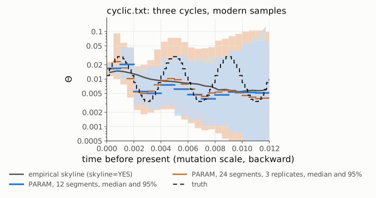
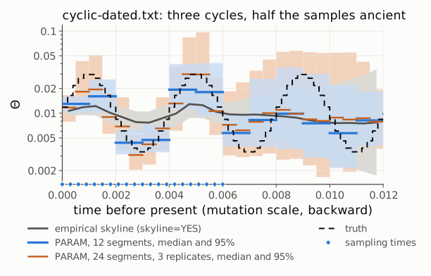
The empirical skylines smooth the cycles into a slow trend (modern) or a damped wave (dated). Segment width matters: the segments here are half a cycle, so the skyline cannot show the peaks themselves (the true Theta reaches 0.03 inside segments whose mean is 0.02).
Narrower segments. cyclic-fine and cyclic-dated-fine halve the
width: 24 segments of 0.0005 (orange in the figures: median and 95%
interval of each segment; the orange bands lie behind the blue ones). Twice
as many segment values need more genealogies per locus for the joint
combination, so these runs use three replicates of every locus chain
(replicate=YES:3), and the dated run also joint-samples=1 (see below).
True value (geometric mean over the segment) and estimate for some
segments:
| Segment | true | cyclic.txt, 24 segments | cyclic-dated.txt, 24 segments |
|---|---|---|---|
| 0.0005-0.0010 (first peak) | 0.027 | 0.023 (0.010-0.092) | 0.018 (0.010-0.043) |
| 0.0025-0.0030 (first trough) | 0.0037 | 0.0050 (0.0018-0.0200) | 0.0031 (0.0020-0.0054) |
| 0.0045-0.0050 (second peak) | 0.027 | 0.010 (0.002-0.074) | 0.030 (0.014-0.084) |
| 0.0065-0.0070 (second trough) | 0.0037 | 0.0046 (0.0009-0.0431) | 0.0062 (0.0029-0.0238) |
| 0.0085-0.0090 (third peak) | 0.027 | 0.0058 (0.0006-0.0702) | 0.0099 (0.0028-0.0575) |
With modern samples the 24 segments reach the first peak (0.023 against 0.027, where the 12-segment value is the segment mean 0.020) and follow the first trough, but from the second peak on the medians stay near the middle and the intervals are wider than with 12 segments: the bottleneck of the first trough leaves too few lineages (see above). With half of the samples ancient the 24 segments show the second cycle as well, peak (0.030 against 0.027) and trough, and the 95% intervals contain the true value in all 24 segments; beyond the oldest sample (t = 0.006) the intervals widen to a factor of 20-30 and the third peak is gone. Each segment holds half the coalescences of a 12-segment run, and the random-walk prior on log tau (section 4) ties neighbouring segments together, so where the data are thin the peaks are smoothed away. The marginal likelihood does not separate the two widths: BTI -19372.7 (24) against -19371.1 (12) for the modern samples, -20549.0 against -20546.1 for the dated ones, all well above constant size (-19407.4 and -20572.7).
The dated run first failed Migrate’s own check of the joint combination.
With 24 segment values the genealogies sampled for a locus must cover a
24-dimensional joint posterior to be reweighted; by default
(joint-samples=AUTO) the combination keeps only as many genealogies per
locus as fit a memory bound (the outfile says “up to … used per locus”),
here 12987 of the 29997 stored, and the median reweighting ESS was 43
(with one replicate 30; the limit is 50). Every value was then marked
Joint*, and the tables and plots used the All values, the product of the
per-locus posteriors. With 20 loci these are much too narrow (a factor of
2-5 everywhere, also far beyond the oldest sample) and missed the true
value in 13 of the 24 segments. joint-samples=1 uses all genealogies
(reweighting ESS 58, no Joint*); the run took 34 instead of 14 min. Look for the * in the Joint rows and the reweighting ESS in
the Monte Carlo error section of the outfile before trusting a
many-segment skyline; with Joint* rows, raise joint-samples or the
number of replicates.
8. Migration through time
skyline-model is laid out like custom-migration: one row per
population, the diagonal for Theta, the off-diagonal entries for the
immigration rates into that population. * gives an entry multipliers,
c keeps it constant (g makes Theta follow population growth, 03-growth;
section 10). For two populations
skyline-model={c * c c} row 1: Theta_1, M_2->1; row 2: M_1->2, Theta_2
lets only M_2->1 (immigration into Arran from Bute) change at
skyline-times={0.003}. Joint estimates (truth in parentheses):
| Parameter | twopop-mig (M_2->1 skyline) | twopop-yes (constant) |
|---|---|---|
| Theta_1 (0.01) | 0.0084 (0.0066-0.0103) | 0.0089 (0.0069-0.0108) |
| Theta_2 (0.005) | 0.0050 (0.0037-0.0063) | 0.0048 (0.0037-0.0060) |
| M_2->1 today (100) | 91 (27-167) | 60 (12-140) |
| M_1->2 (400) | 370 (209-560) | 402 (258-572) |
| tau_2 of M_2->1 (5) | 2.7 (0.40-8.0) | - |
| M_2->1 before 0.003 (500) | 246 (28-665) | - |
| log ML (BTI) | -20261.4 | -20261.1 |
The intervals cover the truth, but they are wide: with 20 loci and 20 sequences per population a five-fold change of a migration rate is not resolved, and the marginal likelihood cannot tell the two models apart. Migration events are few compared with coalescences, so a migration-rate skyline needs more data than a Theta skyline (more loci, more samples) or a larger change.
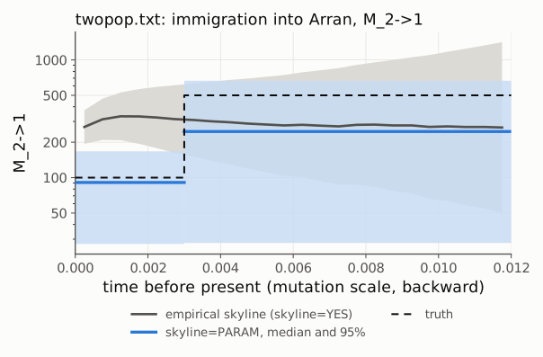
The empirical skyline of M_2->1 (from twopop-yes) stays near 270-320 at
all times, above the Joint estimate: the migrations it counts are those of
each locus’ own genealogies, sampled with that locus’ M, and a single locus
says little about M (its posterior is close to the prior, mean 500). For
weakly informed parameters the empirical skyline therefore reflects the
prior; the joint estimates combine the loci. Before Migrate 7.0.110 and
6.1.86 the joint combination of a migration skyline was wrong (the
multipliers were integrated only within the prior range of M) and gave
values of several thousand; rerun such analyses.
9. Both versions of Migrate
Migrate 6.1.86 gives the same results (MPI runs differ in the order in which the loci are dispatched, so the numbers differ slightly):
| Model | Theta today, 7.0.110 / 6.1.86 | tau_2, 7.0.110 / 6.1.86 |
|---|---|---|
| expand-param | 0.0084 / 0.0084 | 0.29 / 0.28 |
| dated-param | 0.0106 / 0.0104 | 0.17 / 0.17 |
10. What next
- Growth-linked skylines:
skyline-modelentryglets Theta follow the exponential growth of 03-growth instead of free multipliers (Theta(t) = Theta e^(-g t)); the outfile then reports Theta at the start of each segment. - 05-model-selection: marginal likelihoods, heating ladders and Bayes factors in more detail (choosing the number of segments is a model choice).
- Migration skylines on real data: use many loci, check that the joint rows are not starred (Joint*), and compare with a model with constant migration.