06 Assignment: individuals of unknown origin
Draft: work in progress. This recipe is not finished yet; sections may be incomplete and results may change.
Status: draft (2026-11-12), sections 1-7. Run with migrate-n 7.0.111.
Some individuals in a data set may have no known population: a bird caught between forests, a sample with a lost label, a possible migrant. Migrate can estimate where such individuals come from while it estimates the population sizes and migration rates. This recipe shows how to mark them, how to read the assignment table, how well assignment works in simulated data, and applies it to the Taita thrush, a bird living in three forest fragments in Kenya. Read 00-basics and 01-migration first.
Contents
- How assignment works
- Assignment in the infile and the parmfile
- The assignment table
- Simulated data: how often is the assignment right?
- A real data set: the Taita thrush
- All birds unlabelled
- What next
1. How assignment works
An individual without a population is a tip of the genealogy whose population is not fixed. Migrate treats that population as one more unknown of the model: besides the genealogy and the parameters, the MCMC proposes moving the individual (all its gene copies, at every locus) to another population, and accepts or rejects the move like any other change. The genealogy is rebuilt around the moved individual, so its new population must fit the data and the migration events that connect it to the rest of the sample.
The posterior probability that the individual belongs to population j is the fraction of the recorded steps in which it was in j. Migrate counts this per locus; the “All” line combines the loci by multiplying the per-locus probabilities and normalizing, as if each locus were independent evidence with an equal prior chance for every population.
Assignment needs no allele-frequency model and no Hardy-Weinberg equilibrium: the populations are described by their Theta and migration rates, and the individual is assigned to the population whose genealogy it fits best. It also allows for migration: an individual from a population that exchanges many migrants with another is hard to place, and the probabilities say so.
2. Assignment in the infile and the parmfile
In the infile, an individual of unknown origin has a ? as the first
character of its name. It must still be listed under some population; that
population is only the starting point of the chain. In a sequence infile
(from section 4):
3 5 06-assignment M50 rep00
(s500) (s500) (s500) (s500) (s500)
10 Arran
Arr00     GCTGAGGAGTCACGAGAGG...
...
?Col08    GCTGAGGAGTCTCGAGAGG...
?Col09    GCTGAGGAGTCTCGAGAGG...
10 Bute
...
?Col08 and ?Col09 (true population Coll) are listed under Arran. With
one line per individual, all loci of ?Col08 move together. In a
microsatellite infile (section 5) the diploid genotype moves as one.
The parmfile:
| Parmfile line | Meaning |
|---|---|
assign=YES:UNIFORM | assign the ? individuals; a move proposes one of the other populations at random |
assign=YES:FREQ | the same; the move proposes populations in proportion to how often the individual was moved to them during the burn-in (with the matching Hastings correction) |
assign=YES:UNIFORM:{1,2} | only populations 1 and 2 are candidates (for example to exclude an unsampled ancestral population of a divergence model) |
assign=NO | default; ? individuals stay where they are listed |
updatefreq= assignment:0.2 | weight of the assignment move among the genealogy and parameter moves (0.2 is the default) |
With assignment the window move of 01-migration is switched off by default;
updatefreq= window:0.1 switches it on. In the simulations of section 4
(M = 50 and 250, UNIFORM) it gave the same assignments (per-sequence
probabilities within 0.11, median difference 0.002-0.02) and took 1.6
times as long. Everything else is the same as in an ordinary
run; the parameters are estimated with the unknown individuals included,
each in the populations it visits.
3. The assignment table
The outfile ends with the table “Assignment of Individuals to populations” (section 4, M = 50, data set rep00, UNIFORM):
Individual Locus        1     2     3
---------- -------- ----- ----- -----
?Col08             1 0.259 0.203 0.538 [2239/110954 = 0.020180]
?Col08             2 0.058 0.145 0.796 [4968/111755 = 0.044454]
?Col08             3 0.099 0.106 0.795 [4202/110704 = 0.037957]
?Col08             4 0.268 0.222 0.510 [3873/110692 = 0.034989]
?Col08             5 0.161 0.097 0.742 [1967/110559 = 0.017791]
?Col08           All 0.000 0.001 0.999
One line per locus with the posterior probability of each population and, in brackets, the accepted and proposed assignment moves for that locus; then the “All” line over loci. No single locus is sure (0.51-0.80 for population 3, Coll), but all five point the same way, and together they give 0.999. The acceptance of the assignment move is low (2-8% in these runs); each individual must still be moved often enough, so check that the accepted count is in the hundreds.
4. Simulated data: how often is the assignment right?
study/make_study.py simulates three populations (Arran, Bute, Coll;
Theta 0.01 each) with equal migration rates M between all of them, 5 loci of
500 bp and 10 sequences per population. In every population the last two
sequences lose their label and are listed under the next population, so
that the chain starts from a wrong assignment. Three migration levels, ten
data sets each, both proposal modes:
python3 study/make_study.py study      # from cookbooks/06-assignment
# run every study/M<m>/<mode>/repNN/parmfile, then
python3 scripts/score.py study
The runs took about 8 minutes each with 6 MPI processes. For the 60 unlabelled sequences of each migration level and mode (P(true): the “All” probability of the true population):
| M (4Nm) | Mode | Correct | Mean P(true) | P(true) > 0.95 | Correct among P > 0.95 |
|---|---|---|---|---|---|
| 10 (0.1) | FREQ | 100% | 1.00 | 100% | 60 of 60 |
| UNIFORM | 100% | 1.00 | 100% | 60 of 60 | |
| 50 (0.5) | FREQ | 100% | 0.97 | 83% | 50 of 50 |
| UNIFORM | 100% | 0.96 | 82% | 49 of 49 | |
| 250 (2.5) | FREQ | 73% | 0.69 | 28% | 17 of 17 |
| UNIFORM | 78% | 0.72 | 28% | 17 of 17 |
(4Nm = Theta x M, the number of immigrants per generation times four.) With little migration every unlabelled sequence returns to its population, with probabilities near 1. With 4Nm = 2.5 a quarter of them end up in the wrong population, but the probabilities report that uncertainty: the mean probability of the true population (0.69-0.72) is close to the fraction assigned correctly (0.73-0.78), and every assignment with a probability above 0.95 was right. FREQ and UNIFORM give the same results here; with three populations the choice of proposal hardly matters.
5. A real data set: the Taita thrush
The Taita thrush (Turdus helleri) lives only in the cloud-forest fragments of the Taita Hills in south-east Kenya: Chawia, Ngangao and Mbololo. Galbusera et al. (2000) genotyped 155 birds caught in 1996-1999 at seven microsatellite loci, found the three fragments genetically differentiated (Migrate estimated 0.2-4.3 migrants per generation), and found with assignment tests (STRUCTURE and IMMANC) no migrant of the current generation and two or three birds descending from migrants. Their genotypes are not public, but a later study (Cousseau et al. 2025) deposited genotypes from the same fragments on Dryad (doi:10.5061/dryad.bvq83bkkk, CC0), with birds from 1997-1998 and later periods. We use the 1997-1998 birds (for Chawia: before the 2008 translocation of birds from Mbololo), the period of the 2000 study: 21 from Chawia, 54 from Ngangao and 86 from Mbololo, at six loci.
scripts/taita_infile.py writes the infile from the Dryad workbook
(dryad/TT_genotypes.xlsx). The alleles are fragment lengths in base pairs,
so the infile has a #@M line with the repeat length of each locus (2 bp,
4 bp for the tetranucleotide MJG1); genotypes that could not be scored are
?:
3 6 . Taita thrush 1997-98 (Dryad bvq83bkkk)
#@M 2,2,4,2,2,2
21 Chawia
B32910    179.183 219.221 222.230 151.167 115.125 268.274
...
The parmfile (parmfiles/parmfile.taita) is the microsatellite parmfile of
00-basics (Brownian motion model, Theta prior 0-20) with three populations,
the full migration model and assign=YES:UNIFORM.
Which birds are not where they were caught? Every bird must be unlabelled once, but with all birds unlabelled no population would have a fixed member (section 6). We use 10-fold cross-validation: the birds are split into ten groups; in each run one group is unlabelled (and listed under a wrong fragment) and the other nine stay labelled:
for k in 0 1 2 3 4 5 6 7 8 9; do
  mkdir -p cv/fold$k
  python3 scripts/taita_infile.py cv/fold$k/taita.txt --folds 10 --fold $k
  cp parmfiles/parmfile.taita cv/fold$k/parmfile
done
# run each fold, then
python3 scripts/score_taita.py cv
Each fold took 48-71 minutes with 7 MPI processes on a cluster.
| Fragment | Birds | Assigned home (P > 0.5) | Home with P > 0.95 | Mean P(home) |
|---|---|---|---|---|
| Chawia | 21 | 21 | 9 | 0.93 |
| Ngangao | 54 | 49 | 10 | 0.78 |
| Mbololo | 86 | 83 | 57 | 0.92 |
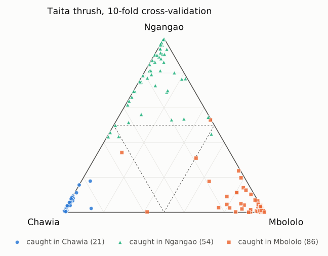
The ternary (de Finetti) diagram (scripts/plot_ternary.py cv OUT.svg)
shows every bird as a point: a bird at a corner belongs to that fragment
with probability 1; the closer a point lies to a corner, the higher that
fragment’s probability. Colour and shape mark the fragment where the bird
was caught; the dashed lines separate the regions in which one fragment has
a probability above 0.5. Most birds sit in or near the corner of their own
fragment. The Ngangao birds spread along the edges toward Chawia and
Mbololo, and a few Mbololo birds lie between Mbololo and the other two.
153 of the 161 birds are assigned to the fragment where they were caught. The eight others are split between two fragments; none is placed elsewhere with a probability above 0.6:
ring       caught in   Chawia  Ngangao  Mbololo
B34139     Mbololo      0.583    0.002    0.415
B34642     Mbololo      0.004    0.530    0.466
BB0386     Mbololo      0.537    0.343    0.119
B34112     Ngangao      0.509    0.435    0.057
B34120     Ngangao      0.560    0.434    0.006
BB0304     Ngangao      0.040    0.449    0.511
BB0329     Ngangao      0.537    0.458    0.004
BB0333     Ngangao      0.493    0.499    0.009
Ngangao is the least distinct fragment (mean probability 0.78; five of its 54 birds lean toward Chawia or Mbololo), Chawia and Mbololo the most. This agrees with Galbusera et al. (2000): no bird is clearly a migrant of the current generation, and a few birds have mixed ancestry. The individual birds cannot be matched to theirs (the 2000 study numbered its samples, Dryad lists ring numbers), so we cannot check whether these are the same birds.
6. All birds unlabelled
What if no bird keeps its label? taita_infile.py --all caught marks
every bird with ? and lists it under the fragment of capture;
--all random lists every bird under a random fragment. Both runs took
about an hour.
The result is uninformative: every bird gets a probability near 1/3 for each fragment (the largest probability of a bird is 0.36-0.55 for 80% of the birds, at most 0.89), and only 8-9 of 161 birds are assigned to the fragment where they were caught. The run that started from the fragments of capture lost them.
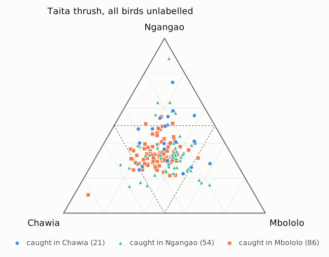
(The run with random starting fragments; the run that started from the fragments of capture looks the same.)
This is expected. With every bird unlabelled, the three population labels are interchangeable: the same three groups with the labels permuted have the same posterior probability (the priors are the same for all populations). A chain that mixes well visits all permutations, and the probability of each bird in each population tends to 1/3, whatever the groups are. The probabilities still differ from 1/3 because one hour of run did not mix completely, not because they say anything about the birds. Assignment in Migrate needs individuals of known origin that fix what each population is; the unlabelled individuals are then compared with those populations. To find groups without any known origin, use a clustering method (for example STRUCTURE) and then test the groups with Migrate.
7. What next
- 05-model-selection: once the origin of the doubtful individuals is settled, compare migration models (full, symmetric, one-way) for the three fragments with marginal likelihoods.
- 07-haplotyping: unphased diploid sequence data, the other case in which the MCMC changes the data side of the genealogy.
References
- Galbusera P, Lens L, Schenck T, Waiyaki E, Matthysen E (2000) Genetic variability and gene flow in the globally, critically-endangered Taita thrush. Conservation Genetics 1: 45-55. doi:10.1023/A:1010184200648
- Cousseau L, Sanczuk P, de Mits S, Vangestel C, Borghesio L, Githiru M, Lens L (2025) Taita thrush genetic and demographic data. Dryad, doi:10.5061/dryad.bvq83bkkk (CC0); article doi:10.1093/ornithapp/duaf010